Train a GCLDA model and use it

This example trains a generalized correspondence latent Dirichlet allocation model using abstracts from Neurosynth and then uses it for decoding.

Warning

The model in this example is trained using (1) a very small, nonrepresentative dataset and (2) very few iterations. As such, it will not provide useful results. If you are interested in using GCLDA, we recommend using a large dataset like Neurosynth, and training with at least 10k iterations.

import os

import numpy as np
import nibabel as nib
from nilearn.plotting import plot_stat_map, plot_roi

import nimare
from nimare import annotate, decode
from nimare.tests.utils import get_test_data_path

Load dataset with abstracts

We’ll load a small dataset composed only of studies in Neurosynth with Angela Laird as a coauthor, for the sake of speed.

dset = nimare.dataset.Dataset.load(
    os.path.join(get_test_data_path(), 'neurosynth_laird_studies.pkl.gz'))

Generate term counts

GCLDA uses raw word counts instead of the tf-idf values generated by Neurosynth.

counts_df = annotate.text.generate_counts(
    dset.texts, text_column='abstract', tfidf=False, max_df=0.99, min_df=0)

Run model

Five iterations will take ~10 minutes with the full Neurosynth dataset. It’s much faster with this reduced example dataset. Note that we’re using only 10 topics here. This is because there are only 13 studies in the dataset. If the number of topics is higher than the number of studies in the dataset, errors can occur during training.

model = annotate.gclda.GCLDAModel(
    counts_df, dset.coordinates, mask=dset.masker.mask_img, n_topics=10)
model.fit(n_iters=100, loglikely_freq=5)
model.save('gclda_model.pkl.gz')

# Let's remove the model now that you know how to generate it.
os.remove('gclda_model.pkl.gz')

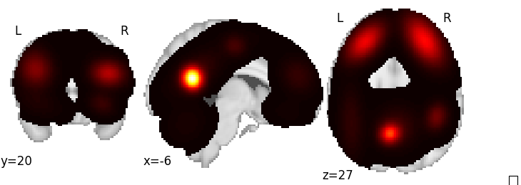
Generate a pseudo-statistic image from text

text = ('anterior cingulate cortex')
encoded_img, _ = decode.encode.gclda_encode(model, text)
plot_stat_map(encoded_img, draw_cross=False)

Out:

<nilearn.plotting.displays.OrthoSlicer object at 0x7f0f799c6da0>

Decode an unthresholded statistical map

For the sake of simplicity, we will use the pseudo-statistic map generated in the previous step.

# Run the decoder
decoded_df, _ = decode.continuous.gclda_decode_map(model, encoded_img)
decoded_df.sort_values(by='Weight', ascending=False).head(10)

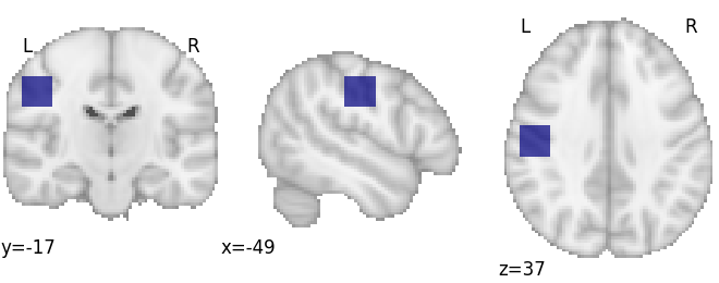
Decode an ROI image

# First we'll make an ROI
arr = np.zeros(dset.masker.mask_img.shape, int)
arr[65:75, 50:60, 50:60] = 1
mask_img = nib.Nifti1Image(arr, dset.masker.mask_img.affine)
plot_roi(mask_img, draw_cross=False)

# Run the decoder
decoded_df, _ = decode.discrete.gclda_decode_roi(model, mask_img)
print(decoded_df.sort_values(by='Weight', ascending=False).head(10))

Out:

               Weight
Term
anterior    21.512598
reasoning   12.387274
speech      10.971806
processes   10.322728
language    10.322728
structural   9.577834
cortex       8.276344
approaches   8.258182
thalamus     8.258182
parietal     8.258182