Machine learning in NiMARE

This example will walk you through some of the typical patterns to work with scikit-learn in NiMARE. You will learn how to:

1. export a Studyset into a scikit-learn dataset.

2. select your feature (what’s doing the predicting) and target (what you want to predict) variables.

3. choose between different kernels and transforms for your model.

4. read a fitted model back onto the brain.

to_bunch() returns a Bunch of the peaks each analysis reported, the study it came from, and an optional target, all in one row order. NiMARE reads the Studyset; scikit-learn handles the rest.

from pathlib import Path

import numpy as np
from nilearn import plotting
from nilearn.datasets import fetch_atlas_difumo
from scipy import sparse
from sklearn.decomposition import TruncatedSVD
from sklearn.feature_selection import VarianceThreshold
from sklearn.impute import SimpleImputer
from sklearn.linear_model import LogisticRegression
from sklearn.model_selection import GroupKFold, GroupShuffleSplit, cross_val_score
from sklearn.pipeline import make_pipeline
from sklearn.preprocessing import OneHotEncoder
from sklearn.random_projection import SparseRandomProjection

from nimare.extract import fetch_neurostore
from nimare.meta.kernel import MKDAKernel
from nimare.ml import (
    MAKernel,
    MaskerTransformer,
    clear_map_cache,
    coefficient_image,
    describe_fields,
    make_nimare_column_transformer,
)
from nimare.nimads import Studyset
from nimare.utils import get_resource_path

RANDOM_SEED = 13
N_COMPONENTS = 64

Load the n-back/flanker Studyset

The bundled Studyset contains coordinate-based analyses of n-back and flanker tasks from NeuroStore. Its parquet tables are loaded from the accompanying studyset.json manifest.

studyset_dir = Path(get_resource_path()) / "nback_vs_flanker_studyset_2026-07"
studyset = Studyset(studyset_dir)

print(f"Studyset: {studyset.name}")
print(f"Analyses: {len(studyset.ids)} from {len(studyset.study_ids)} studies")
print(studyset.metadata["comparison_task"].value_counts().to_string())

Studyset: n-back vs flanker task analysis examples
Analyses: 906 from 320 studies
comparison_task
n-back     500
flanker    406

Build the feature set

to_bunch() reads each analysis’s foci into a row of peak counts over the image grid, and reads the comparison_task metadata field as the "n-back" and "flanker" labels to predict. Name a field either way: a bare field name, or a (source, field) pair when the same name appears in more than one Studyset table.

You choose the kernel later, in the pipeline, so that it is fitted on training rows only and can be tuned like any other step.

bunch = studyset.to_bunch(
    target_field=("metadata", "comparison_task"),
    # Hold out a quarter of the studies; see the next section.
    test_size=0.25,
    random_state=RANDOM_SEED,
)

print(f"Feature data: {bunch.data.shape}, sparse={bunch.data.format}")
print(f"Non-zeros: {bunch.data.nnz:,} peaks")
print(f"Labels: {sorted(set(bunch.target))}")
print(f"Dropped studies because of no coordinates: {len(bunch.provenance['dropped_ids'])}")

Feature data: (906, 902629), sparse=csr
Non-zeros: 9,359 peaks
Labels: ['flanker', 'n-back']
Dropped studies because of no coordinates: 0

If you’ve worked with scikit-learn, bunch may be familiar: sparse data, aligned target, and groups holding the study each analysis came from. It also carries ids, feature_names, voxel_columns, descriptor_columns, descriptor_names, the masker whose grid the voxels span, and provenance.

The voxel columns span the whole image grid. A coordinate just outside the mask still spreads into it once a kernel is applied, so the full grid keeps that contribution.

print(f"Bunch: {', '.join(sorted(bunch))}")

Bunch: data, descriptor_categories, descriptor_columns, descriptor_names, feature_names, groups, ids, masker, provenance, target, test, train, voxel_columns

Split testing and training at the study level, not the analysis level

Analyses from one study are related, so keep each study on one side of the split. Passing test_size above added train and test row positions to the bunch, grouped by study. test_size counts studies, so the analysis counts approximate the fraction you asked for.

train, test = bunch.train, bunch.test

print(f"Train: {len(train)} analyses from {len(set(bunch.groups[train]))} studies")
print(f"Test:  {len(test)} analyses from {len(set(bunch.groups[test]))} studies")
print(f"Shared studies: {set(bunch.groups[train]) & set(bunch.groups[test])}")

Train: 686 analyses from 240 studies
Test:  220 analyses from 80 studies
Shared studies: set()

The split is a GroupShuffleSplit over groups. For several splits of one bunch, or for cross-validation, convert once and hand groups to a group splitter.

Classify the task label

bunch.data is an ordinary sparse matrix, so an ordinary scikit-learn pipeline works on it. MAKernel turns the peaks into MA maps as the first step, truncated SVD reduces them before the classifier sees them, and both are fitted on training rows only because they are in the pipeline. GroupKFold reads the same study labels the split used.

Every column here is a voxel, so each step can see the whole matrix. The section after next adds descriptor columns and gives each block its own transformer.

cache=True reuses maps the kernel has already made. An MA map depends only on that analysis’s own peaks, so the row made for one fold is the row the next fold needs.

pipeline = make_pipeline(
    MAKernel(MKDAKernel(r=10), source_masker=bunch.masker, cache=True),
    TruncatedSVD(n_components=50, random_state=RANDOM_SEED),
    LogisticRegression(max_iter=1000, class_weight="balanced", random_state=RANDOM_SEED),
)
scores = cross_val_score(
    pipeline,
    bunch.data,
    bunch.target,
    cv=GroupKFold(5),
    groups=bunch.groups,
)

print(f"Cross-validation accuracy: {scores.mean():.3f} +/- {scores.std():.3f}")

Cross-validation accuracy: 0.623 +/- 0.030

interpret the model results in the brain

The classifier weighs SVD components, and you want to know which regions carry the prediction. coefficient_image() walks the fitted pipeline backwards, undoing each reduction until the weights are one per voxel, and unmasks them into an image. The walk stops at the kernel, whose input is peaks.

Fit on every row here. The folds above gave you the accuracy; this is the map the model would carry into use.

pipeline.fit(bunch.data, bunch.target)
weights = coefficient_image(pipeline, bunch)

print(f"Weight image: {weights.shape}")
print(f"Positive weights favour: {pipeline[-1].classes_[1]}")

plotting.plot_stat_map(
    weights,
    display_mode="z",
    cut_coords=5,
    title=f"{pipeline[-1].classes_[1]} versus {pipeline[-1].classes_[0]}",
)

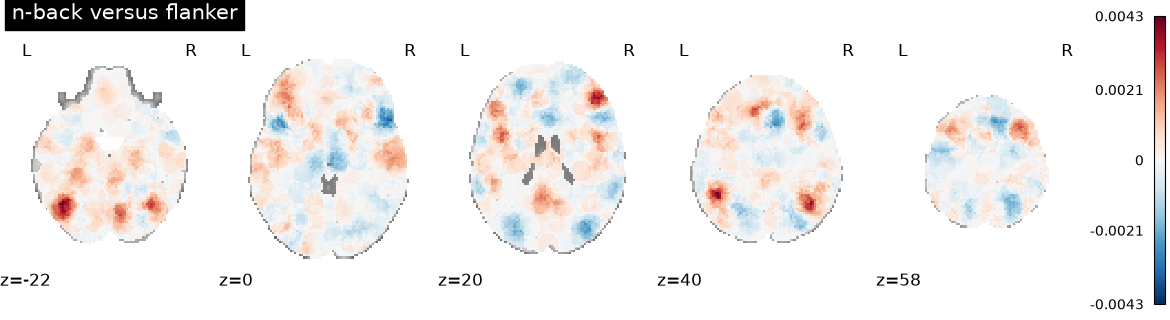
Weight image: (91, 109, 91)
Positive weights favour: n-back

<nilearn.plotting.displays._slicers.ZSlicer object at 0x7ff9bd26bc20>

The cached maps are held for the process, which is what lets each fold’s clone reuse them. clear_map_cache() releases them and reports what they served. They grow to the size of the feature matrix, so release them when you move on to another studyset.

print(f"Map cache: {clear_map_cache()}")

Map cache: {'rows': 894, 'hits': 4542, 'misses': 894}

Add study information as extra features

Numeric metadata and annotation fields can be appended to the feature matrix as extra columns. You have explicit control on how to handle missing data: by default a field that some analyses leave out stops the conversion and names them, so the choice stays yours. Pass missing_values="drop" to remove those analyses, or "keep" to leave the gaps for an imputer in your pipeline.

try:
    studyset.to_bunch(descriptor_fields=["sample_sizes"])
except ValueError as exc:
    print(f"{str(exc)[:160]}...")

Missing values in sample_sizes (904 analyses: '25uKFzHufiGk-MwAgKDUaAoMn', '2DMUS9MeRxqW-8yjf2zEWEJgv', '2DMUS9MeRxqW-XSvaHoFaRbV5', ... (904 total)). Fix the S...

Once there are descriptor columns, give each block its own transformer so it works on the voxels only. That is what ColumnTransformer is for, and make_nimare_column_transformer() is make_column_transformer() with the bunch filled in. Pass (transformer, columns) pairs as scikit-learn takes them, where columns may be "voxels", "descriptors", or a descriptor’s own field name. It binds the bunch’s masker into an atlas, keeps the column names so a coefficient reads back to its field, and picks a sparse_threshold that keeps a wide voxel block sparse.

A transformer per descriptor is just another pair: (SimpleImputer(), "sample_sizes"), (StandardScaler(), "year"). For anything this does not cover, write out bunch.voxel_columns and bunch.descriptor_columns, which are ordinary slices.

with_descriptors = studyset.to_bunch(
    target_field=("metadata", "comparison_task"),
    descriptor_fields=["sample_sizes"],
    missing_values="keep",
)
preprocessor = make_nimare_column_transformer(
    with_descriptors,
    (
        make_pipeline(
            MAKernel(MKDAKernel(r=10), source_masker=with_descriptors.masker),
            TruncatedSVD(n_components=50, random_state=RANDOM_SEED),
        ),
        "voxels",
    ),
    (SimpleImputer(strategy="median"), "descriptors"),
)

print(f"Descriptors: {with_descriptors.descriptor_names}")
print(f"Descriptor columns: {with_descriptors.descriptor_columns}")
print(f"With descriptors: {type(preprocessor).__name__}")
print(f"Steps: {[name for name, _, _ in preprocessor.transformers]}")

Descriptors: ['sample_sizes']
Descriptor columns: slice(902629, 902630, None)
With descriptors: ColumnTransformer
Steps: ['pipeline', 'simpleimputer']

Use a categorical field as a feature

Categorical features are represented numerically through category codes, and descriptor_categories tells you how the codes relate back to the categories. Pick your category encoder in the pipeline, and treat it like any other scikit-learn transformer.

The bunch fills in the two things scikit-learn works out from a frame but not from an array of numbers: categories=, so a training split that happens to miss a category still yields the same number of columns, and the real labels in get_feature_names_out. A code stands for a label, so give it an encoder.

GROUP = "ParticipantDemographicsExtractor.groups[0].group_name"
with_group = studyset.to_bunch(
    target_field=("metadata", "comparison_task"),
    descriptor_fields=[("annotations", GROUP)],
    missing_values={"target": "drop", "descriptors": "keep"},
)
encoded = make_nimare_column_transformer(
    with_group,
    ("drop", "voxels"),
    (OneHotEncoder(handle_unknown="ignore"), GROUP),
).fit(with_group.data)

print(f"Categories: {with_group.descriptor_categories}")
print(f"Encoded as: {[n.split('.')[-1] for n in encoded.get_feature_names_out()]}")

try:
    make_nimare_column_transformer(with_group, ("drop", "voxels"), ("passthrough", GROUP))
except ValueError as exc:
    print(f"{str(exc)[:150]}...")

Categories: {'ParticipantDemographicsExtractor.groups[0].group_name': ['healthy', 'patients']}
Encoded as: ['group_name_healthy', 'group_name_patients']
'ParticipantDemographicsExtractor.groups[0].group_name' is a coded categorical descriptor and cannot be passed through: its values are positions in bu...

Select annotation labels

Annotations usually run to thousands of labels, so a glob pattern takes them all, each under its own name, reading from the Studyset’s sparse label block. A label no analysis carries is a zero, so a pattern selection gives you a complete label matrix.

neurosynth = Studyset(str(Path(get_resource_path()) / "neurosynth_laird_studyset.json"))
annotated = neurosynth.to_bunch(
    descriptor_fields=[("annotations", "Neurosynth_TFIDF__*")],
)

labels = annotated.data[:, annotated.descriptor_columns]
print(f"Bunch: {annotated.data.shape}, of which labels: {labels.shape[1]}")
print(f"Non-zero labels: {labels.nnz}")
print(f"Names kept whole: {annotated.descriptor_names[:2]}")
print(f"Still sparse: {sparse.issparse(annotated.data)}")

Bunch: (17, 905857), of which labels: 3228
Non-zero labels: 1167
Names kept whole: ['Neurosynth_TFIDF__001', 'Neurosynth_TFIDF__01']
Still sparse: True

Compare transformer workflows

Any scikit-learn transformer that reads sparse input will do, downstream of the kernel: truncated SVD, sparse random projection, variance thresholding and atlas aggregation all do. PCA reads sparse input through its arpack or covariance_eigh solvers and centres the data, so truncated SVD is the usual choice for a matrix this wide.

transformers = {
    "Truncated SVD": TruncatedSVD(n_components=N_COMPONENTS, random_state=RANDOM_SEED),
    "Sparse random projection": SparseRandomProjection(
        n_components=N_COMPONENTS, random_state=RANDOM_SEED
    ),
    "Variance threshold": VarianceThreshold(threshold=0.01),
}
splitter = GroupShuffleSplit(n_splits=1, test_size=0.2, random_state=RANDOM_SEED)

for name, transformer in transformers.items():
    reduced_pipeline = make_pipeline(
        MAKernel(MKDAKernel(r=10), source_masker=bunch.masker),
        transformer,
        LogisticRegression(max_iter=1000, class_weight="balanced", random_state=RANDOM_SEED),
    )
    score = cross_val_score(
        reduced_pipeline,
        bunch.data,
        bunch.target,
        cv=splitter,
        groups=bunch.groups,
    )[0]
    print(f"{name} grouped holdout accuracy: {score:.3f}")

Truncated SVD grouped holdout accuracy: 0.605
Sparse random projection grouped holdout accuracy: 0.593
Variance threshold grouped holdout accuracy: 0.679

Let nilearn transform the voxels

A nilearn masker is already a scikit-learn transformer, and it takes images where a ColumnTransformer hands out columns of an array. MaskerTransformer bridges the two, using the bunch’s masker to know which voxel each column is.

It applies any nilearn masker, or anything nilearn loads as an atlas: what a fetch_atlas_* function returns, an atlas image or file, or a fetcher name such as "harvard_oxford". A 4D atlas is summarised with a NiftiMapsMasker and a 3D one with a NiftiLabelsMasker, and the atlas’s own region names become the feature names. A NiftiMasker gives you voxels back, which is how nilearn’s smoothing and standardizing reach these features:

(NiftiMasker(smoothing_fwhm=6), "voxels")

It reads either column space, working it out from the width: the bunch’s raw peak columns, which gives the coordinates reported per region, or the MA maps a kernel made, as here.

Outside a pipeline, fit the transformer on the training rows and apply that same fitted one to the held-out rows.

difumo = fetch_atlas_difumo(dimension=N_COMPONENTS, resolution_mm=2)
atlas_transformer = MaskerTransformer(difumo, source_masker=bunch.masker)

maps = MAKernel(MKDAKernel(r=10), source_masker=bunch.masker).fit_transform(
    bunch.data[:, bunch.voxel_columns]
)
train_reduced = atlas_transformer.fit_transform(maps[train])
test_reduced = atlas_transformer.transform(maps[test])

print(f"Reduced train features: {train_reduced.shape}")
print(f"Reduced test features:  {test_reduced.shape}")
# get_feature_names_out follows scikit-learn and returns an array of numpy
# strings; tolist() gives the plain ones.
print(f"First region names: {atlas_transformer.get_feature_names_out()[:3].tolist()}")

model = LogisticRegression(max_iter=1000, class_weight="balanced", random_state=RANDOM_SEED)
model.fit(train_reduced, bunch.target[train])

print(f"DiFuMo holdout accuracy: {model.score(test_reduced, bunch.target[test]):.3f}")

[fetch_atlas_difumo] Added README.md to /home/docs/nilearn_data
[fetch_atlas_difumo] Dataset created in /home/docs/nilearn_data/difumo_atlases
[fetch_atlas_difumo] Downloading data from https://osf.io/pqu9r/download ...
[fetch_atlas_difumo]  ...done. (7 seconds, 0 min)

[fetch_atlas_difumo] Extracting data from
/home/docs/nilearn_data/difumo_atlases/4658bee5f4fab958dab48d7fa59e6e62/download
...
[fetch_atlas_difumo] .. done.

[fetch_atlas_difumo] Downloading data from https://osf.io/4k9bf/download ...
[fetch_atlas_difumo]  ...done. (1 seconds, 0 min)

Reduced train features: (686, 64)
Reduced test features:  (220, 64)
First region names: ['Superior frontal sulcus', 'Fusiform gyrus', 'Calcarine cortex posterior']
DiFuMo holdout accuracy: 0.559

Work with a release-scale Studyset

fetch_neurostore() downloads a published NeuroStore release, annotated with hundreds of labels by LLM extractors. The same three steps work on any Studyset large enough that reading its field list by hand is impractical.

studyset = fetch_neurostore(version="2026-09")

print(f"Analyses: {len(studyset.ids)} from {len(set(studyset.study_ids))} studies")

Analyses: 115748 from 32444 studies

Ask which fields are usable

describe_fields() reports every field a selector may name, with the kind to_bunch() will read it as and the fraction of analyses reporting it. Most of a release is a long tail, so picking a field becomes a query.

all_fields = describe_fields(studyset)
fields = all_fields[all_fields.coverage >= 0.5]
targets = fields[fields.n_unique.between(2, 12)]

print(f"Fields at >=50% coverage: {len(fields)} of {len(all_fields)}")
print(targets[["source", "field", "kind", "coverage", "n_unique"]].to_string(index=False))

Fields at >=50% coverage: 29 of 997
     source                                                     field        kind  coverage  n_unique
annotations     ParticipantDemographicsExtractor.groups[0].group_name categorical  0.933796         3
annotations ParticipantDemographicsExtractor.groups[0].imaging_sample categorical  0.933588         2
   metadata                                                    source categorical  0.863920         4
annotations                   TaskExtractor.fMRITasks[0].RestingState     numeric  0.813526         2

Convert the part you are modelling

Conversion reads peaks, so a whole release converts in a couple of seconds. Applying the kernel is the expensive step, so slice the Studyset to the analyses you are modelling first: slice() takes analysis ids. missing_values="drop" removes the analyses the extractor left blank.

subset = studyset.slice(analyses=list(studyset.ids)[:4000])
resting = subset.to_bunch(
    target_field=("annotations", "TaskExtractor.fMRITasks[0].RestingState"),
    missing_values="drop",
)

print(f"Kept {resting.data.shape[0]} of {len(subset.ids)} analyses")
print(f"Resting-state rows: {int(np.sum(np.asarray(resting.target) == 1.0))}")

Kept 3141 of 4000 analyses
Resting-state rows: 445

An extractor’s repeated fields are indexed, and brackets are glob syntax, so *groups[0].* is retried with its brackets taken literally and selects group zero as intended. That group mixes numeric and categorical labels, so filter the field column to kind == "numeric" for the descriptor list.

demographics = fields[
    (fields.kind == "numeric") & fields.field.str.contains("groups[0].", regex=False)
]
with_demographics = subset.to_bunch(
    target_field=("annotations", "TaskExtractor.fMRITasks[0].RestingState"),
    descriptor_fields=[("annotations", name) for name in demographics.field],
    # A descriptor gap an imputer can fill; a target gap it cannot, so the two
    # roles get different policies.
    missing_values={"target": "drop", "descriptors": "keep"},
)

print(f"Bunch: {with_demographics.data.shape}")
print(f"Descriptors: {[name.split('.')[-1] for name in with_demographics.descriptor_names]}")

Bunch: (3141, 902635)
Descriptors: ['count', 'female_count', 'male_count', 'age_mean', 'age_minimum', 'age_maximum']

Classify resting-state against task

From here it is the workflow above: a grouped split so each study stays on one side, and an imputer for the descriptor gaps the "descriptors": "keep" policy left for the pipeline.

Resting-state analyses are the minority here, so use roc_auc: it asks whether the foci rank a resting-state analysis above a task one.

release_pipeline = make_pipeline(
    make_nimare_column_transformer(
        with_demographics,
        (
            make_pipeline(
                MAKernel(MKDAKernel(r=10), source_masker=with_demographics.masker),
                TruncatedSVD(n_components=50, random_state=RANDOM_SEED),
            ),
            "voxels",
        ),
        (SimpleImputer(strategy="median"), "descriptors"),
    ),
    LogisticRegression(max_iter=1000, class_weight="balanced", random_state=RANDOM_SEED),
)
release_bunch = with_demographics
release_scores = cross_val_score(
    release_pipeline,
    release_bunch.data,
    release_bunch.target,
    cv=GroupKFold(5),
    groups=release_bunch.groups,
    scoring="roc_auc",
)

n_resting = int(np.sum(release_bunch.target == 1.0))

print(f"Resting-state rows: {n_resting} of {len(release_bunch.target)}")
print(f"Resting-state ROC AUC: {release_scores.mean():.3f} +/- {release_scores.std():.3f}")

Resting-state rows: 445 of 3141
Resting-state ROC AUC: 0.664 +/- 0.014