Note
Click here to download the full example code
Subtraction and conjunction CBMAs
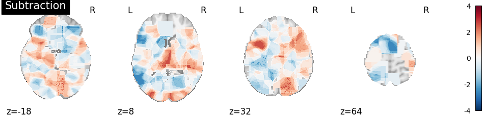
The (coordinate-based) ALE subtraction method tests at which voxels the meta-analytic results from two groups of studies differ reliably from one another. 1, 2
import os

import matplotlib.pyplot as plt
from nilearn.image import math_img
from nilearn.plotting import plot_stat_map

from nimare import io, utils
from nimare.correct import FWECorrector
from nimare.diagnostics import Jackknife
from nimare.meta.cbma import ALE, ALESubtraction
Load Sleuth text files into Datasets
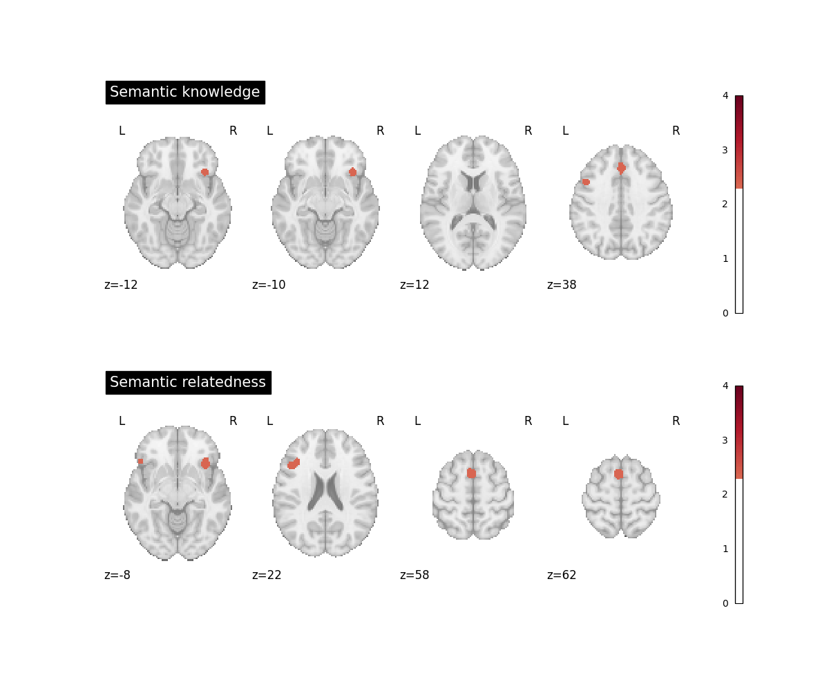
The data for this example are a subset of studies from a meta-analysis on semantic cognition in children. 3 A first group of studies probed children’s semantic world knowledge (e.g., correctly naming an object after hearing its auditory description) while a second group of studies asked children to decide if two (or more) words were semantically related to one another or not.
knowledge_file = os.path.join(utils.get_resource_path(), "semantic_knowledge_children.txt")
related_file = os.path.join(utils.get_resource_path(), "semantic_relatedness_children.txt")

knowledge_dset = io.convert_sleuth_to_dataset(knowledge_file)
related_dset = io.convert_sleuth_to_dataset(related_file)
Individual group ALEs
Computing separate ALE analyses for each group is not strictly necessary for performing the subtraction analysis but will help the experimenter to appreciate the similarities and differences between the groups.
ale = ALE(null_method="approximate")
knowledge_results = ale.fit(knowledge_dset)
related_results = ale.fit(related_dset)

corr = FWECorrector(method="montecarlo", voxel_thresh=0.001, n_iters=100, n_cores=1)
knowledge_corrected_results = corr.transform(knowledge_results)
related_corrected_results = corr.transform(related_results)

fig, axes = plt.subplots(figsize=(12, 10), nrows=2)
img = knowledge_corrected_results.get_map("z_desc-size_level-cluster_corr-FWE_method-montecarlo")
plot_stat_map(
    img,
    cut_coords=4,
    display_mode="z",
    title="Semantic knowledge",
    threshold=2.326,  # cluster-level p < .01, one-tailed
    cmap="RdBu_r",
    vmax=4,
    axes=axes[0],
    figure=fig,
)

img2 = related_corrected_results.get_map("z_desc-size_level-cluster_corr-FWE_method-montecarlo")
plot_stat_map(
    img2,
    cut_coords=4,
    display_mode="z",
    title="Semantic relatedness",
    threshold=2.326,  # cluster-level p < .01, one-tailed
    cmap="RdBu_r",
    vmax=4,
    axes=axes[1],
    figure=fig,
)
fig.show()
Out:
  0%|          | 0/100 [00:00<?, ?it/s]
  1%|1         | 1/100 [00:00<00:40,  2.44it/s]
  2%|2         | 2/100 [00:00<00:39,  2.45it/s]
  3%|3         | 3/100 [00:01<00:39,  2.45it/s]
  4%|4         | 4/100 [00:01<00:39,  2.44it/s]
  5%|5         | 5/100 [00:02<00:38,  2.44it/s]
  6%|6         | 6/100 [00:02<00:38,  2.45it/s]
  7%|7         | 7/100 [00:02<00:37,  2.45it/s]
  8%|8         | 8/100 [00:03<00:37,  2.45it/s]
  9%|9         | 9/100 [00:03<00:37,  2.45it/s]
 10%|#         | 10/100 [00:04<00:37,  2.42it/s]
 11%|#1        | 11/100 [00:04<00:36,  2.42it/s]
 12%|#2        | 12/100 [00:04<00:36,  2.42it/s]
 13%|#3        | 13/100 [00:05<00:35,  2.43it/s]
 14%|#4        | 14/100 [00:05<00:35,  2.43it/s]
 15%|#5        | 15/100 [00:06<00:34,  2.44it/s]
 16%|#6        | 16/100 [00:06<00:34,  2.44it/s]
 17%|#7        | 17/100 [00:06<00:33,  2.45it/s]
 18%|#8        | 18/100 [00:07<00:33,  2.44it/s]
 19%|#9        | 19/100 [00:07<00:33,  2.44it/s]
 20%|##        | 20/100 [00:08<00:32,  2.45it/s]
 21%|##1       | 21/100 [00:08<00:32,  2.45it/s]
 22%|##2       | 22/100 [00:09<00:31,  2.45it/s]
 23%|##3       | 23/100 [00:09<00:31,  2.45it/s]
 24%|##4       | 24/100 [00:09<00:31,  2.45it/s]
 25%|##5       | 25/100 [00:10<00:30,  2.45it/s]
 26%|##6       | 26/100 [00:10<00:30,  2.45it/s]
 27%|##7       | 27/100 [00:11<00:29,  2.44it/s]
 28%|##8       | 28/100 [00:11<00:29,  2.45it/s]
 29%|##9       | 29/100 [00:11<00:29,  2.45it/s]
 30%|###       | 30/100 [00:12<00:28,  2.45it/s]
 31%|###1      | 31/100 [00:12<00:28,  2.45it/s]
 32%|###2      | 32/100 [00:13<00:27,  2.45it/s]
 33%|###3      | 33/100 [00:13<00:27,  2.45it/s]
 34%|###4      | 34/100 [00:13<00:26,  2.45it/s]
 35%|###5      | 35/100 [00:14<00:26,  2.45it/s]
 36%|###6      | 36/100 [00:14<00:26,  2.45it/s]
 37%|###7      | 37/100 [00:15<00:25,  2.45it/s]
 38%|###8      | 38/100 [00:15<00:25,  2.45it/s]
 39%|###9      | 39/100 [00:15<00:24,  2.45it/s]
 40%|####      | 40/100 [00:16<00:24,  2.45it/s]
 41%|####1     | 41/100 [00:16<00:24,  2.45it/s]
 42%|####2     | 42/100 [00:17<00:23,  2.45it/s]
 43%|####3     | 43/100 [00:17<00:23,  2.45it/s]
 44%|####4     | 44/100 [00:17<00:22,  2.45it/s]
 45%|####5     | 45/100 [00:18<00:22,  2.45it/s]
 46%|####6     | 46/100 [00:18<00:22,  2.44it/s]
 47%|####6     | 47/100 [00:19<00:21,  2.44it/s]
 48%|####8     | 48/100 [00:19<00:21,  2.44it/s]
 49%|####9     | 49/100 [00:20<00:20,  2.44it/s]
 50%|#####     | 50/100 [00:20<00:20,  2.44it/s]
 51%|#####1    | 51/100 [00:20<00:20,  2.44it/s]
 52%|#####2    | 52/100 [00:21<00:19,  2.45it/s]
 53%|#####3    | 53/100 [00:21<00:19,  2.45it/s]
 54%|#####4    | 54/100 [00:22<00:18,  2.45it/s]
 55%|#####5    | 55/100 [00:22<00:18,  2.45it/s]
 56%|#####6    | 56/100 [00:22<00:17,  2.45it/s]
 57%|#####6    | 57/100 [00:23<00:17,  2.45it/s]
 58%|#####8    | 58/100 [00:23<00:17,  2.44it/s]
 59%|#####8    | 59/100 [00:24<00:16,  2.44it/s]
 60%|######    | 60/100 [00:24<00:16,  2.44it/s]
 61%|######1   | 61/100 [00:24<00:15,  2.45it/s]
 62%|######2   | 62/100 [00:25<00:15,  2.45it/s]
 63%|######3   | 63/100 [00:25<00:15,  2.45it/s]
 64%|######4   | 64/100 [00:26<00:14,  2.45it/s]
 65%|######5   | 65/100 [00:26<00:14,  2.45it/s]
 66%|######6   | 66/100 [00:26<00:13,  2.44it/s]
 67%|######7   | 67/100 [00:27<00:13,  2.45it/s]
 68%|######8   | 68/100 [00:27<00:13,  2.45it/s]
 69%|######9   | 69/100 [00:28<00:12,  2.45it/s]
 70%|#######   | 70/100 [00:28<00:12,  2.45it/s]
 71%|#######1  | 71/100 [00:29<00:11,  2.45it/s]
 72%|#######2  | 72/100 [00:29<00:11,  2.45it/s]
 73%|#######3  | 73/100 [00:29<00:11,  2.45it/s]
 74%|#######4  | 74/100 [00:30<00:10,  2.45it/s]
 75%|#######5  | 75/100 [00:30<00:10,  2.45it/s]
 76%|#######6  | 76/100 [00:31<00:09,  2.45it/s]
 77%|#######7  | 77/100 [00:31<00:09,  2.45it/s]
 78%|#######8  | 78/100 [00:31<00:08,  2.45it/s]
 79%|#######9  | 79/100 [00:32<00:08,  2.45it/s]
 80%|########  | 80/100 [00:32<00:08,  2.46it/s]
 81%|########1 | 81/100 [00:33<00:07,  2.46it/s]
 82%|########2 | 82/100 [00:33<00:07,  2.46it/s]
 83%|########2 | 83/100 [00:33<00:06,  2.45it/s]
 84%|########4 | 84/100 [00:34<00:06,  2.46it/s]
 85%|########5 | 85/100 [00:34<00:06,  2.46it/s]
 86%|########6 | 86/100 [00:35<00:05,  2.45it/s]
 87%|########7 | 87/100 [00:35<00:05,  2.45it/s]
 88%|########8 | 88/100 [00:35<00:04,  2.45it/s]
 89%|########9 | 89/100 [00:36<00:04,  2.44it/s]
 90%|######### | 90/100 [00:36<00:04,  2.44it/s]
 91%|#########1| 91/100 [00:37<00:03,  2.44it/s]
 92%|#########2| 92/100 [00:37<00:03,  2.45it/s]
 93%|#########3| 93/100 [00:38<00:02,  2.44it/s]
 94%|#########3| 94/100 [00:38<00:02,  2.44it/s]
 95%|#########5| 95/100 [00:38<00:02,  2.44it/s]
 96%|#########6| 96/100 [00:39<00:01,  2.44it/s]
 97%|#########7| 97/100 [00:39<00:01,  2.44it/s]
 98%|#########8| 98/100 [00:40<00:00,  2.44it/s]
 99%|#########9| 99/100 [00:40<00:00,  2.44it/s]
100%|##########| 100/100 [00:40<00:00,  2.44it/s]
100%|##########| 100/100 [00:40<00:00,  2.45it/s]

  0%|          | 0/100 [00:00<?, ?it/s]
  1%|1         | 1/100 [00:00<00:35,  2.76it/s]
  2%|2         | 2/100 [00:00<00:35,  2.79it/s]
  3%|3         | 3/100 [00:01<00:34,  2.80it/s]
  4%|4         | 4/100 [00:01<00:34,  2.80it/s]
  5%|5         | 5/100 [00:01<00:33,  2.80it/s]
  6%|6         | 6/100 [00:02<00:33,  2.80it/s]
  7%|7         | 7/100 [00:02<00:33,  2.80it/s]
  8%|8         | 8/100 [00:02<00:32,  2.81it/s]
  9%|9         | 9/100 [00:03<00:32,  2.80it/s]
 10%|#         | 10/100 [00:03<00:31,  2.81it/s]
 11%|#1        | 11/100 [00:03<00:31,  2.82it/s]
 12%|#2        | 12/100 [00:04<00:31,  2.82it/s]
 13%|#3        | 13/100 [00:04<00:30,  2.82it/s]
 14%|#4        | 14/100 [00:04<00:30,  2.83it/s]
 15%|#5        | 15/100 [00:05<00:30,  2.83it/s]
 16%|#6        | 16/100 [00:05<00:29,  2.82it/s]
 17%|#7        | 17/100 [00:06<00:29,  2.82it/s]
 18%|#8        | 18/100 [00:06<00:29,  2.81it/s]
 19%|#9        | 19/100 [00:06<00:28,  2.81it/s]
 20%|##        | 20/100 [00:07<00:28,  2.81it/s]
 21%|##1       | 21/100 [00:07<00:28,  2.80it/s]
 22%|##2       | 22/100 [00:07<00:27,  2.81it/s]
 23%|##3       | 23/100 [00:08<00:27,  2.81it/s]
 24%|##4       | 24/100 [00:08<00:27,  2.80it/s]
 25%|##5       | 25/100 [00:08<00:26,  2.80it/s]
 26%|##6       | 26/100 [00:09<00:26,  2.80it/s]
 27%|##7       | 27/100 [00:09<00:26,  2.81it/s]
 28%|##8       | 28/100 [00:09<00:25,  2.80it/s]
 29%|##9       | 29/100 [00:10<00:25,  2.80it/s]
 30%|###       | 30/100 [00:10<00:24,  2.80it/s]
 31%|###1      | 31/100 [00:11<00:24,  2.79it/s]
 32%|###2      | 32/100 [00:11<00:24,  2.79it/s]
 33%|###3      | 33/100 [00:11<00:24,  2.79it/s]
 34%|###4      | 34/100 [00:12<00:23,  2.79it/s]
 35%|###5      | 35/100 [00:12<00:23,  2.79it/s]
 36%|###6      | 36/100 [00:12<00:22,  2.79it/s]
 37%|###7      | 37/100 [00:13<00:22,  2.80it/s]
 38%|###8      | 38/100 [00:13<00:22,  2.81it/s]
 39%|###9      | 39/100 [00:13<00:21,  2.81it/s]
 40%|####      | 40/100 [00:14<00:21,  2.81it/s]
 41%|####1     | 41/100 [00:14<00:21,  2.81it/s]
 42%|####2     | 42/100 [00:14<00:20,  2.81it/s]
 43%|####3     | 43/100 [00:15<00:20,  2.80it/s]
 44%|####4     | 44/100 [00:15<00:20,  2.80it/s]
 45%|####5     | 45/100 [00:16<00:19,  2.80it/s]
 46%|####6     | 46/100 [00:16<00:19,  2.80it/s]
 47%|####6     | 47/100 [00:16<00:18,  2.80it/s]
 48%|####8     | 48/100 [00:17<00:18,  2.81it/s]
 49%|####9     | 49/100 [00:17<00:18,  2.80it/s]
 50%|#####     | 50/100 [00:17<00:17,  2.80it/s]
 51%|#####1    | 51/100 [00:18<00:17,  2.81it/s]
 52%|#####2    | 52/100 [00:18<00:17,  2.81it/s]
 53%|#####3    | 53/100 [00:18<00:16,  2.81it/s]
 54%|#####4    | 54/100 [00:19<00:16,  2.81it/s]
 55%|#####5    | 55/100 [00:19<00:16,  2.81it/s]
 56%|#####6    | 56/100 [00:19<00:15,  2.81it/s]
 57%|#####6    | 57/100 [00:20<00:15,  2.80it/s]
 58%|#####8    | 58/100 [00:20<00:14,  2.81it/s]
 59%|#####8    | 59/100 [00:21<00:14,  2.82it/s]
 60%|######    | 60/100 [00:21<00:14,  2.82it/s]
 61%|######1   | 61/100 [00:21<00:13,  2.82it/s]
 62%|######2   | 62/100 [00:22<00:13,  2.81it/s]
 63%|######3   | 63/100 [00:22<00:13,  2.81it/s]
 64%|######4   | 64/100 [00:22<00:12,  2.81it/s]
 65%|######5   | 65/100 [00:23<00:12,  2.82it/s]
 66%|######6   | 66/100 [00:23<00:12,  2.81it/s]
 67%|######7   | 67/100 [00:23<00:11,  2.81it/s]
 68%|######8   | 68/100 [00:24<00:11,  2.81it/s]
 69%|######9   | 69/100 [00:24<00:11,  2.81it/s]
 70%|#######   | 70/100 [00:24<00:10,  2.81it/s]
 71%|#######1  | 71/100 [00:25<00:10,  2.81it/s]
 72%|#######2  | 72/100 [00:25<00:09,  2.81it/s]
 73%|#######3  | 73/100 [00:26<00:09,  2.81it/s]
 74%|#######4  | 74/100 [00:26<00:09,  2.80it/s]
 75%|#######5  | 75/100 [00:26<00:08,  2.80it/s]
 76%|#######6  | 76/100 [00:27<00:08,  2.80it/s]
 77%|#######7  | 77/100 [00:27<00:08,  2.79it/s]
 78%|#######8  | 78/100 [00:27<00:07,  2.79it/s]
 79%|#######9  | 79/100 [00:28<00:07,  2.80it/s]
 80%|########  | 80/100 [00:28<00:07,  2.80it/s]
 81%|########1 | 81/100 [00:28<00:06,  2.79it/s]
 82%|########2 | 82/100 [00:29<00:06,  2.80it/s]
 83%|########2 | 83/100 [00:29<00:06,  2.80it/s]
 84%|########4 | 84/100 [00:29<00:05,  2.80it/s]
 85%|########5 | 85/100 [00:30<00:05,  2.81it/s]
 86%|########6 | 86/100 [00:30<00:04,  2.81it/s]
 87%|########7 | 87/100 [00:31<00:04,  2.81it/s]
 88%|########8 | 88/100 [00:31<00:04,  2.80it/s]
 89%|########9 | 89/100 [00:31<00:03,  2.80it/s]
 90%|######### | 90/100 [00:32<00:03,  2.80it/s]
 91%|#########1| 91/100 [00:32<00:03,  2.81it/s]
 92%|#########2| 92/100 [00:32<00:02,  2.81it/s]
 93%|#########3| 93/100 [00:33<00:02,  2.81it/s]
 94%|#########3| 94/100 [00:33<00:02,  2.80it/s]
 95%|#########5| 95/100 [00:33<00:01,  2.81it/s]
 96%|#########6| 96/100 [00:34<00:01,  2.80it/s]
 97%|#########7| 97/100 [00:34<00:01,  2.80it/s]
 98%|#########8| 98/100 [00:34<00:00,  2.80it/s]
 99%|#########9| 99/100 [00:35<00:00,  2.80it/s]
100%|##########| 100/100 [00:35<00:00,  2.81it/s]
100%|##########| 100/100 [00:35<00:00,  2.81it/s]
Characterize the relative contributions of experiments in the ALE results
jknife = Jackknife(
    target_image="z_desc-size_level-cluster_corr-FWE_method-montecarlo",
    voxel_thresh=None,
)
knowledge_cluster_table, knowledge_cluster_img = jknife.transform(knowledge_corrected_results)
related_cluster_table, related_cluster_img = jknife.transform(related_corrected_results)
Out:
  0%|          | 0/21 [00:00<?, ?it/s]
  5%|4         | 1/21 [00:01<00:35,  1.77s/it]
 10%|9         | 2/21 [00:03<00:32,  1.69s/it]
 14%|#4        | 3/21 [00:05<00:29,  1.67s/it]
 19%|#9        | 4/21 [00:06<00:28,  1.65s/it]
 24%|##3       | 5/21 [00:08<00:26,  1.64s/it]
 29%|##8       | 6/21 [00:09<00:24,  1.64s/it]
 33%|###3      | 7/21 [00:11<00:22,  1.63s/it]
 38%|###8      | 8/21 [00:13<00:21,  1.63s/it]
 43%|####2     | 9/21 [00:14<00:19,  1.63s/it]
 48%|####7     | 10/21 [00:16<00:17,  1.63s/it]
 52%|#####2    | 11/21 [00:18<00:16,  1.63s/it]
 57%|#####7    | 12/21 [00:19<00:14,  1.63s/it]
 62%|######1   | 13/21 [00:21<00:13,  1.63s/it]
 67%|######6   | 14/21 [00:22<00:11,  1.63s/it]
 71%|#######1  | 15/21 [00:24<00:09,  1.63s/it]
 76%|#######6  | 16/21 [00:26<00:08,  1.63s/it]
 81%|########  | 17/21 [00:27<00:06,  1.63s/it]
 86%|########5 | 18/21 [00:29<00:04,  1.63s/it]
 90%|######### | 19/21 [00:31<00:03,  1.63s/it]
 95%|#########5| 20/21 [00:32<00:01,  1.63s/it]
100%|##########| 21/21 [00:34<00:00,  1.63s/it]
100%|##########| 21/21 [00:34<00:00,  1.64s/it]

  0%|          | 0/16 [00:00<?, ?it/s]
  6%|6         | 1/16 [00:01<00:24,  1.63s/it]
 12%|#2        | 2/16 [00:03<00:21,  1.53s/it]
 19%|#8        | 3/16 [00:04<00:19,  1.50s/it]
 25%|##5       | 4/16 [00:06<00:17,  1.49s/it]
 31%|###1      | 5/16 [00:07<00:16,  1.48s/it]
 38%|###7      | 6/16 [00:08<00:14,  1.47s/it]
 44%|####3     | 7/16 [00:10<00:13,  1.46s/it]
 50%|#####     | 8/16 [00:11<00:11,  1.46s/it]
 56%|#####6    | 9/16 [00:13<00:10,  1.46s/it]
 62%|######2   | 10/16 [00:14<00:08,  1.46s/it]
 69%|######8   | 11/16 [00:16<00:07,  1.46s/it]
 75%|#######5  | 12/16 [00:17<00:05,  1.46s/it]
 81%|########1 | 13/16 [00:19<00:04,  1.46s/it]
 88%|########7 | 14/16 [00:20<00:02,  1.46s/it]
 94%|#########3| 15/16 [00:22<00:01,  1.46s/it]
100%|##########| 16/16 [00:23<00:00,  1.45s/it]
100%|##########| 16/16 [00:23<00:00,  1.47s/it]
Subtraction analysis
Typically, one would use at least 10000 iterations for a subtraction analysis. However, we have reduced this to 100 iterations for this example.
sub = ALESubtraction(n_iters=100, memory_limit=None)
res_sub = sub.fit(knowledge_dset, related_dset)
img_sub = res_sub.get_map("z_desc-group1MinusGroup2")

plot_stat_map(
    img_sub,
    cut_coords=4,
    display_mode="z",
    title="Subtraction",
    cmap="RdBu_r",
    vmax=4,
)
Out:
<nilearn.plotting.displays.ZSlicer object at 0x7fab56a69290>
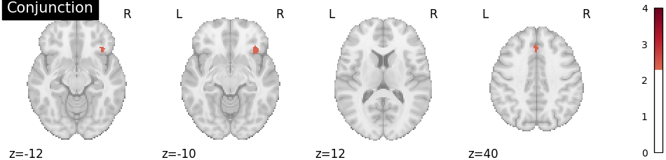
Conjunction analysis
To determine the overlap of the meta-analytic results, a conjunction image
can be computed by (a) identifying voxels that were statistically significant
in both individual group maps and (b) selecting, for each of these voxels,
the smaller of the two group-specific z values. 4 Since this is simple
arithmetic on images, conjunction is not implemented as a separate method in
NiMARE but can easily be achieved with nilearn.image.math_img().
Out:
<nilearn.plotting.displays.ZSlicer object at 0x7fab3eca1050>
References
- 1
Laird, Angela R., et al. “ALE meta‐analysis: Controlling the false discovery rate and performing statistical contrasts.” Human brain mapping 25.1 (2005): 155-164. https://doi.org/10.1002/hbm.20136
- 2
Eickhoff, Simon B., et al. “Activation likelihood estimation meta-analysis revisited.” Neuroimage 59.3 (2012): 2349-2361. https://doi.org/10.1016/j.neuroimage.2011.09.017
- 3
Enge, Alexander, et al. “A meta-analysis of fMRI studies of semantic cognition in children.” Neuroimage 241 (2021): 118436. https://doi.org/10.1016/j.neuroimage.2021.118436
- 4
Nichols, Thomas, et al. “Valid conjunction inference with the minimum statistic.” Neuroimage 25.3 (2005): 653-660. https://doi.org/10.1016/j.neuroimage.2004.12.005
Total running time of the script: ( 2 minutes 40.449 seconds)