Sample-size weighting in MKDA

Weighting each study contrast by the square root of its sample size is what the “multilevel” in Multilevel Kernel Density Analysis refers to. A contrast from 90 subjects says more about the population than one from 9, and MKDA encodes that by weighting the contrast indicator maps before averaging them [1][2]:

where is the contrast’s sample size and optionally discounts contrasts analysed with a fixed-effects study-level model.

This example shows how to turn the weighting on and what it changes in the map.

Weighting is opt-in: MKDADensity with no arguments weights every contrast equally, so existing analyses are unaffected.

Load a Studyset

Weighting needs a sample size for every contrast. The NIDM pain Studyset shipped with NiMARE records one.

import os

import numpy as np
import pandas as pd
from nilearn.plotting import plot_stat_map

from nimare.meta.cbma import MKDADensity
from nimare.meta.cbma.weights import StudyWeights, normalize_weights
from nimare.nimads import Studyset
from nimare.utils import get_resource_path

studyset_file = os.path.join(get_resource_path(), "nidm_pain_studyset.json")
studyset = Studyset(studyset_file, target="mni152_2mm")

sample_sizes = {
    row["id"]: int(np.mean(row["sample_sizes"]))
    for _, row in studyset.metadata.iterrows()
    if isinstance(row["sample_sizes"], (list, tuple, np.ndarray))
}
print(
    f"{len(studyset.ids)} contrasts, "
    f"sample sizes {min(sample_sizes.values())}-{max(sample_sizes.values())}"
)

21 contrasts, sample sizes 9-32

The default: every contrast weighted equally

MKDADensity() gives every contrast a weight of exactly 1.0, so its summary statistic is the count of contrasts activating a voxel.

unweighted = MKDADensity(kernel__r=10.0)
res_unweighted = unweighted.fit(studyset)

weights = np.asarray(unweighted.weight_vec_).ravel()
print("distinct weights:", np.unique(weights))
print("sum:", weights.sum(), "= number of contrasts")

distinct weights: [1.]
sum: 21.0 = number of contrasts

Turning the weighting on

weighting="sample_size" is shorthand for StudyWeights(), which reads the collection’s sample_sizes metadata and applies .

weighted = MKDADensity(weighting="sample_size", kernel__r=10.0)
res_weighted = weighted.fit(studyset)

ids = list(weighted.inputs_["id"])
table = pd.DataFrame(
    {
        "id": ids,
        "N": [sample_sizes[study_id] for study_id in ids],
        "weight": np.asarray(weighted.weight_vec_).ravel(),
    }
)
table["sqrt_N"] = np.sqrt(table["N"])

print(f"weights sum to {table['weight'].sum():.6f} (= {len(table)} contrasts)")
print(
    f"spread: {table['weight'].min():.4f} to {table['weight'].max():.4f}, "
    f"a factor of {table['weight'].max() / table['weight'].min():.2f}"
)
print(table.sort_values("N").head(8).to_string(index=False))

weights sum to 21.000000 (= 21 contrasts)
spread: 0.7648 to 1.4421, a factor of 1.89
            id  N   weight   sqrt_N
pain_06.nidm-1  9 0.764808 3.000000
pain_07.nidm-1  9 0.764808 3.000000
pain_05.nidm-1  9 0.764808 3.000000
pain_08.nidm-1 12 0.883125 3.464102
pain_10.nidm-1 12 0.883125 3.464102
pain_11.nidm-1 12 0.883125 3.464102
pain_09.nidm-1 12 0.883125 3.464102
pain_17.nidm-1 12 0.883125 3.464102

The weights are normalised to sum to the number of contrasts, so an unweighted analysis is the special case where all of them are 1.0. That keeps the statistic on the same scale either way; dividing by the contrast count recovers the weighted proportion of Wager et al.[2].

Note the weights go as , not as . The largest study here has 3.6x the subjects of the smallest but only 1.9x the weight, which is the point of the square root: it keeps one large study from dominating the map.

ratio = table["weight"] / table["sqrt_N"]
print(f"weight / sqrt(N) is constant: {ratio.min():.9f} to {ratio.max():.9f}")

weight / sqrt(N) is constant: 0.254936105 to 0.254936105

What it changes in the map

Weighting moves which voxels come out on top, because a cluster supported by three small studies now counts for less than one supported by three large ones.

for name, result in [("Unweighted", res_unweighted), ("sqrt(N) weighted", res_weighted)]:
    plot_stat_map(
        result.get_map("z"),
        cut_coords=[0, 0, -8],
        draw_cross=False,
        cmap="RdBu_r",
        symmetric_cbar=True,
        threshold=1.65,
        title=name,
    )

• 
• 

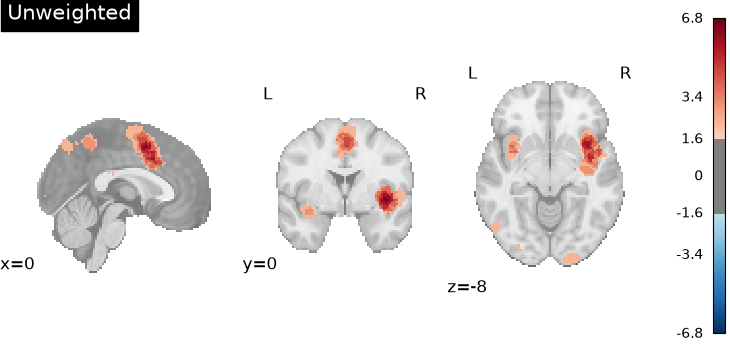
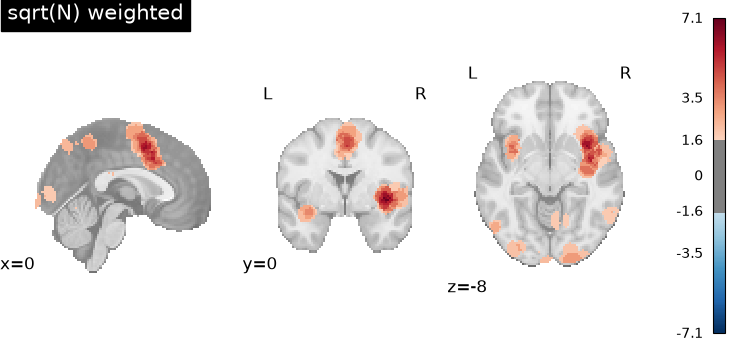
The two maps are highly correlated – weighting rescales the same contrasts rather than changing which ones enter – but the ranking of voxels does move, and as a consequence different voxels may survive the threshold.

stat_u = unweighted.masker.transform(res_unweighted.get_map("stat")).ravel()
stat_w = weighted.masker.transform(res_weighted.get_map("stat")).ravel()

both = (stat_u > 0) | (stat_w > 0)
print(f"Pearson r : {np.corrcoef(stat_u[both], stat_w[both])[0, 1]:.6f}")
print(
    "Spearman  : "
    f"{pd.Series(stat_u[both]).corr(pd.Series(stat_w[both]), method='spearman'):.6f}"
)
print(f"peak      : {stat_u.max():.4f} unweighted vs {stat_w.max():.4f} weighted")

Pearson r : 0.987008
Spearman  : 0.870224
peak      : 10.0000 unweighted vs 10.4868 weighted

Other ways to set the weights

StudyWeights covers the variations of the published method. Pass one instead of the "sample_size" shorthand.

# sqrt(N) is the published transform; "linear" weights by N itself, which is not
# what Wager et al. describe.
linear = StudyWeights(transform="linear")

# Wager et al. discount fixed-effects contrasts. Name the metadata field that records
# each contrast's study-level model; contrasts it does not label are left alone. This
# Studyset has no such field, so the discount is only shown, not applied below --
# NiMARE will not guess which contrasts were fixed-effects, because guessing wrong
# biases every voxel.
ffx = StudyWeights(inference_field="inference", fixed_effects_discount=0.75)
print(f"fixed-effects discount: {ffx.fixed_effects_discount} on field {ffx.inference_field!r}")

# Explicit per-study weights bypass the sample size entirely -- the route for the
# "other study quality measures" the paper mentions.
explicit = StudyWeights(source={study_id: 1.0 for study_id in studyset.ids})

for name, spec in [("sqrt(N)", StudyWeights()), ("linear N", linear), ("explicit", explicit)]:
    raw = spec.raw_weights(studyset, ids)
    w = normalize_weights(raw.to_numpy(), len(ids))
    print(f"{name:10s} min={w.min():.4f} max={w.max():.4f} sum={w.sum():.4f}")

fixed-effects discount: 0.75 on field 'inference'
sqrt(N)    min=0.7648 max=1.4421 sum=21.0000
linear N   min=0.5659 max=2.0120 sum=21.0000
explicit   min=1.0000 max=1.0000 sum=21.0000

When sample sizes are missing

A contrast with a missing or non-positive sample size raises by default, because a substituted weight is invisible in the output map.

incomplete = studyset.to_dict()
incomplete["studies"][0]["analyses"][0]["metadata"]["sample_sizes"] = None
incomplete = Studyset(incomplete, target="mni152_2mm")

try:
    MKDADensity(weighting="sample_size").fit(incomplete)
except ValueError as exc:
    print(f"ValueError: {exc}")

ValueError: 1 contrast has a missing or non-positive weight: pain_01.nidm-1. Populate their sample sizes, or pass StudyWeights(on_missing='impute') to give them the mean weight.

Pass on_missing="impute" to give those contrasts the mean weight of the rest instead, which is what the CanLab implementation does. It keeps the weighted and unweighted analyses over the same study set, at the cost of weighting some contrasts by a number that is not theirs.

imputing = StudyWeights(on_missing="impute")
raw = imputing.raw_weights(incomplete, list(incomplete.ids))
print(f"{imputing.n_imputed_} contrast(s) imputed, weight {raw.iloc[0]:.4f}")

1 contrast(s) imputed, weight 3.8687

References

[1]

Tor D Wager, Martin Lindquist, and Lauren Kaplan. Meta-analysis of functional neuroimaging data: current and future directions. Social cognitive and affective neuroscience, 2(2):150–158, 2007. URL: https://doi.org/10.1093/scan/nsm015, doi:10.1093/scan/nsm015.

[2] (1,2)

Tor D Wager, Martin A Lindquist, Thomas E Nichols, Hedy Kober, and Jared X Van Snellenberg. Evaluating the consistency and specificity of neuroimaging data using meta-analysis. NeuroImage, 45(1 Suppl):S210–S221, 2009. URL: https://doi.org/10.1016/j.neuroimage.2008.10.061, doi:10.1016/j.neuroimage.2008.10.061.