Note
Go to the end to download the full example code.
Stability diagnostics: Jackknife vs. ResampledStability
Once a meta-analysis has been run and a thresholded result is in hand, the natural next question is: how much should we trust it? NiMARE provides two post-hoc diagnostics that approach this question from complementary angles.
Jackknife asks “which studies are responsible for each
significant cluster?” It loops through every study, refits the meta-analysis without
that study, and reports how much the cluster-level statistics drop — a high contribution
score means the cluster depends heavily on a single experiment.
ResampledStability asks “how reproducibly does each brain
voxel survive thresholding when we perturb the study set?” It generates many resampled
versions of the dataset, refits the full pipeline on each, and averages the binary
significant/not-significant outcome across resamples — yielding a voxelwise stability map
between 0 (never significant) and 1 (always significant).
The two diagnostics measure different things and have different computational costs:
Jackknife is fast (N refits for N studies), cluster-level, and study-level — ideal as a first robustness check built into every workflow.
ResampledStability is spatially explicit, voxelwise, and policy-flexible — better suited for publication-quality robustness figures and large-dataset analyses.
This example runs both on the same ALE result so you can compare their outputs directly.
Note
For real analyses use n_iters ≥ 5000 for the FWE corrector and
n_resamples ≥ 100 for ResampledStability.
We use small counts here purely for documentation-build speed.
Imports and constants
import copy
import os
import warnings

import matplotlib.pyplot as plt
import pandas as pd
from nilearn.plotting import plot_stat_map

from nimare.correct import FWECorrector
from nimare.diagnostics import Jackknife, ResampledStability
from nimare.meta.cbma.ale import ALE
from nimare.nimads import Studyset
from nimare.utils import get_resource_path

warnings.filterwarnings("ignore")

N_ITERS = 50       # increase to ≥5000 for real analyses
N_RESAMPLES = 20   # increase to ≥100 for real analyses
RANDOM_STATE = 42
Load data and fit the baseline ALE meta-analysis
We use the NiMARE pain dataset (21 studies, MNI 2 mm) throughout this
example. Both diagnostics operate on an already-fitted
MetaResult, so we run ALE and apply a Monte Carlo
FWE corrector once and then reuse that result for each diagnostic.
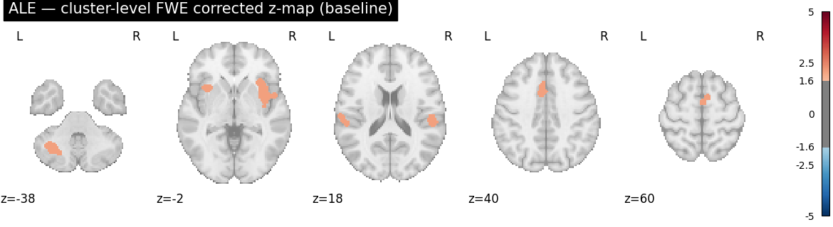
The cluster-level corrected z-map is our primary target image — the one that determines which voxels are “significant” and therefore which clusters the diagnostics evaluate.
studyset_file = os.path.join(get_resource_path(), "nidm_pain_studyset.json")
studyset = Studyset(studyset_file, target="mni152_2mm")
print(f"Number of studies: {len(studyset.studies)}")

ale = ALE()
result = ale.fit(studyset)

corrector = FWECorrector(method="montecarlo", n_iters=N_ITERS, n_cores=1)
result = corrector.transform(result)

TARGET_IMAGE = "z_desc-size_level-cluster_corr-FWE_method-montecarlo"
Number of studies: 21

  0%|          | 0/50 [00:00<?, ?it/s]
  4%|▍         | 2/50 [00:00<00:02, 17.94it/s]
  8%|▊         | 4/50 [00:00<00:02, 17.70it/s]
 12%|█▏        | 6/50 [00:00<00:02, 17.60it/s]
 16%|█▌        | 8/50 [00:00<00:02, 17.57it/s]
 20%|██        | 10/50 [00:00<00:02, 17.61it/s]
 24%|██▍       | 12/50 [00:00<00:02, 17.50it/s]
 28%|██▊       | 14/50 [00:00<00:02, 17.57it/s]
 32%|███▏      | 16/50 [00:00<00:01, 17.60it/s]
 36%|███▌      | 18/50 [00:01<00:01, 17.65it/s]
 40%|████      | 20/50 [00:01<00:01, 17.73it/s]
 44%|████▍     | 22/50 [00:01<00:01, 17.76it/s]
 48%|████▊     | 24/50 [00:01<00:01, 17.68it/s]
 52%|█████▏    | 26/50 [00:01<00:01, 17.76it/s]
 56%|█████▌    | 28/50 [00:01<00:01, 17.70it/s]
 60%|██████    | 30/50 [00:01<00:01, 17.72it/s]
 64%|██████▍   | 32/50 [00:01<00:01, 17.84it/s]
 68%|██████▊   | 34/50 [00:01<00:00, 17.90it/s]
 72%|███████▏  | 36/50 [00:02<00:00, 17.89it/s]
 76%|███████▌  | 38/50 [00:02<00:00, 17.92it/s]
 80%|████████  | 40/50 [00:02<00:00, 17.88it/s]
 84%|████████▍ | 42/50 [00:02<00:00, 17.92it/s]
 88%|████████▊ | 44/50 [00:02<00:00, 17.95it/s]
 92%|█████████▏| 46/50 [00:02<00:00, 17.95it/s]
 96%|█████████▌| 48/50 [00:02<00:00, 17.99it/s]
100%|██████████| 50/50 [00:02<00:00, 18.07it/s]
100%|██████████| 50/50 [00:02<00:00, 17.80it/s]
Baseline corrected result
Before running any diagnostics, we visualise the cluster-level FWE-corrected z-map. This is the map that the diagnostics will characterise.
plot_stat_map(
    result.get_map(TARGET_IMAGE),
    cut_coords=5,
    display_mode="z",
    title="ALE — cluster-level FWE corrected z-map (baseline)",
    threshold=1.65,
    cmap="RdBu_r",
    symmetric_cbar=True,
    vmax=5,
)
plt.show()
Jackknife: identifying influential studies
Jackknife characterises each study’s
proportional contribution to every significant cluster.
For each study i the algorithm:
Refits the estimator on all remaining N − 1 studies.
Computes the proportional reduction in the summary statistic at each voxel:
1 − (stat_{−i} / stat_full).Averages across all voxels in the cluster.
A contribution near 1 means removing study i substantially reduces the cluster statistic — that study is a strong driver. A contribution near 0 means the cluster survives almost unchanged without it.
Because Jackknife only recomputes the summary statistic (not the full Monte
Carlo null distribution) for each N − 1 dataset, it is comparatively fast.
It is the default diagnostic in CBMAWorkflow
and IBMAWorkflow.
jackknife = Jackknife(target_image=TARGET_IMAGE, n_cores=1)
result_jk = jackknife.transform(copy.deepcopy(result))
  0%|          | 0/21 [00:00<?, ?it/s]
  5%|▍         | 1/21 [00:00<00:05,  3.62it/s]
 10%|▉         | 2/21 [00:00<00:05,  3.61it/s]
 14%|█▍        | 3/21 [00:00<00:04,  3.60it/s]
 19%|█▉        | 4/21 [00:01<00:04,  3.60it/s]
 24%|██▍       | 5/21 [00:01<00:04,  3.57it/s]
 29%|██▊       | 6/21 [00:01<00:04,  3.52it/s]
 33%|███▎      | 7/21 [00:01<00:03,  3.51it/s]
 38%|███▊      | 8/21 [00:02<00:03,  3.53it/s]
 43%|████▎     | 9/21 [00:02<00:03,  3.55it/s]
 48%|████▊     | 10/21 [00:02<00:03,  3.55it/s]
 52%|█████▏    | 11/21 [00:03<00:02,  3.54it/s]
 57%|█████▋    | 12/21 [00:03<00:02,  3.56it/s]
 62%|██████▏   | 13/21 [00:03<00:02,  3.56it/s]
 67%|██████▋   | 14/21 [00:03<00:01,  3.54it/s]
 71%|███████▏  | 15/21 [00:04<00:01,  3.55it/s]
 76%|███████▌  | 16/21 [00:04<00:01,  3.56it/s]
 81%|████████  | 17/21 [00:04<00:01,  3.57it/s]
 86%|████████▌ | 18/21 [00:05<00:00,  3.57it/s]
 90%|█████████ | 19/21 [00:05<00:00,  3.58it/s]
 95%|█████████▌| 20/21 [00:05<00:00,  3.58it/s]
100%|██████████| 21/21 [00:05<00:00,  3.57it/s]
100%|██████████| 21/21 [00:05<00:00,  3.56it/s]
Jackknife clusters table
The clusters table summarises the location and size of each significant cluster. Peak statistic and MNI centre of mass are reported for each.
clust_key = f"{TARGET_IMAGE}_tab-clust"
result_jk.tables[clust_key]
Jackknife study-contribution table
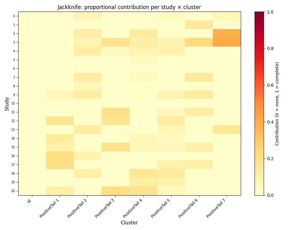
Each row is a study; each column is a cluster. Cell values are the mean proportional contribution of that study to that cluster. High values (e.g. > 0.8) flag studies whose removal would substantially weaken a cluster — worth inspecting for outlier coordinates, inflated sample sizes, or duplicate peaks.
contrib_key = f"{TARGET_IMAGE}_diag-Jackknife_tab-counts_tail-positive"
contrib_df = result_jk.tables.get(contrib_key)
contrib_df
Visualise study contributions as a heatmap
A heatmap makes it easy to spot studies that dominate one or more clusters and studies that contribute little across the board. If a single row shows consistently high values, the corresponding study warrants closer scrutiny.
if contrib_df is not None and not contrib_df.empty:
    contrib_values = contrib_df.apply(pd.to_numeric, errors="coerce").fillna(0.0)
    fig, ax = plt.subplots(
        figsize=(
            max(6, len(contrib_values.columns) * 1.2),
            max(5, len(contrib_values) * 0.35),
        )
    )
    im = ax.imshow(
        contrib_values.to_numpy(dtype=float),
        aspect="auto",
        cmap="YlOrRd",
        vmin=0,
        vmax=1,
    )
    ax.set_xticks(range(len(contrib_values.columns)))
    ax.set_xticklabels(contrib_values.columns, rotation=45, ha="right", fontsize=9)
    ax.set_yticks(range(len(contrib_values)))
    ax.set_yticklabels(contrib_values.index, fontsize=7)
    ax.set_xlabel("Cluster", fontsize=11)
    ax.set_ylabel("Study", fontsize=11)
    ax.set_title("Jackknife: proportional contribution per study × cluster", fontsize=12)
    plt.colorbar(im, ax=ax, label="Contribution (0 = none, 1 = complete)")
    plt.tight_layout()
    plt.show()

    mean_contrib = contrib_values.mean(axis=1).sort_values(ascending=False)
    print("Mean contribution across all clusters (top 10):")
    print(mean_contrib.head(10).to_string())
else:
    print("No clusters found — increase N_ITERS or lower the cluster threshold.")
Mean contribution across all clusters (top 10):
3     0.134950
2     0.081439
20    0.068167
15    0.062635
12    0.058094
17    0.051781
9     0.050901
18    0.048890
11    0.046178
13    0.043190
ResampledStability: voxelwise reproducibility under resampling
ResampledStability estimates how reliably each
voxel survives thresholding when the composition of the study set changes.
For each replicate the algorithm:
Draws a subset of studies according to the chosen
resampling_policy.Refits the full estimator (and corrector, if the target image requires it) on the subset.
Thresholds the result and records a binary support map (1 = significant, 0 = not).
The final stability map is the mean binary support across all replicates. A stability of 1 means the voxel survived thresholding in every replicate; a stability of 0 means it never survived.
Three resampling policies are available:
"leave_1_out"— omit exactly one study per replicate; deterministic; generates N replicates for N studies."leave_k_out"— omit k studies per replicate; useful for testing sensitivity to blocks of studies."subsample"— random subsamples oftarget_nstudies; flexible and recommended for large datasets (> 30 studies).
Unlike Jackknife, ResampledStability does not identify which study is responsible for instability — it only tells you where the result is stable. The two diagnostics are therefore complementary: run Jackknife first to flag influential studies, then add ResampledStability to document spatial reliability for publication.
Leave-one-out stability
"leave_1_out" is the most conservative policy: it drops exactly one study
per replicate, giving N deterministic replicates. Because every study is
omitted exactly once, the result is fully reproducible without a random seed.
This policy is recommended for small datasets (< 25 studies) where removing a
single study can substantially change the analysis.
rs_loo = ResampledStability(
    target_image=TARGET_IMAGE,
    resampling_policy="leave_1_out",
    n_cores=1,
)
result_loo = rs_loo.transform(copy.deepcopy(result))

print("Leave-one-out summary:")
print(result_loo.tables[f"{TARGET_IMAGE}_diag-ResampledStability_tab-summary"])
  0%|          | 0/21 [00:00<?, ?it/s]
 24%|██▍       | 5/21 [00:00<00:00, 45.08it/s]
 48%|████▊     | 10/21 [00:00<00:00, 44.71it/s]
 71%|███████▏  | 15/21 [00:00<00:00, 44.92it/s]
 95%|█████████▌| 20/21 [00:00<00:00, 45.12it/s]
100%|██████████| 21/21 [00:00<00:00, 45.06it/s]
Leave-one-out summary:
                                        target_image  ... random_state
0  z_desc-size_level-cluster_corr-FWE_method-mont...  ...         None

[1 rows x 6 columns]
Leave-k-out stability
"leave_k_out" omits k studies per replicate. This tests whether the
result is stable under a more substantial perturbation than leaving one study
out — useful when you suspect that a block of methodologically similar
studies (e.g. the same lab, the same paradigm) may be jointly driving a
cluster. Set n_resamples to control how many random subsets are drawn.
rs_lko = ResampledStability(
    target_image=TARGET_IMAGE,
    resampling_policy="leave_k_out",
    k=3,
    n_resamples=N_RESAMPLES,
    random_state=RANDOM_STATE,
    n_cores=1,
)
result_lko = rs_lko.transform(copy.deepcopy(result))

print(f"Leave-{rs_lko.k}-out summary:")
print(result_lko.tables[f"{TARGET_IMAGE}_diag-ResampledStability_tab-summary"])
  0%|          | 0/20 [00:00<?, ?it/s]
 25%|██▌       | 5/20 [00:00<00:00, 47.34it/s]
 50%|█████     | 10/20 [00:00<00:00, 47.40it/s]
 75%|███████▌  | 15/20 [00:00<00:00, 47.42it/s]
100%|██████████| 20/20 [00:00<00:00, 47.28it/s]
100%|██████████| 20/20 [00:00<00:00, 47.29it/s]
Leave-3-out summary:
                                        target_image  ... random_state
0  z_desc-size_level-cluster_corr-FWE_method-mont...  ...           42

[1 rows x 6 columns]
Subsample stability
"subsample" draws random subsets of target_n studies. The subsetting
fraction controls the stringency: subsampling at 50 % is a harder test than
90 %. A common choice is 75–80 % of the available studies, which retains
enough power to detect real effects while exposing sensitivity to individual
studies. This policy is the most general and is recommended for larger
datasets where exhaustive leave-k-out enumeration would be prohibitive.
n_studies = len(studyset.studies)
target_n = max(3, int(n_studies * 0.75))  # 75 % of available studies

rs_sub = ResampledStability(
    target_image=TARGET_IMAGE,
    resampling_policy="subsample",
    target_n=target_n,
    n_resamples=N_RESAMPLES,
    random_state=RANDOM_STATE,
    n_cores=1,
)
result_sub = rs_sub.transform(copy.deepcopy(result))

print(f"Subsample (n={target_n}) summary:")
print(result_sub.tables[f"{TARGET_IMAGE}_diag-ResampledStability_tab-summary"])
  0%|          | 0/20 [00:00<?, ?it/s]
 25%|██▌       | 5/20 [00:00<00:00, 46.86it/s]
 55%|█████▌    | 11/20 [00:00<00:00, 49.10it/s]
 85%|████████▌ | 17/20 [00:00<00:00, 50.06it/s]
100%|██████████| 20/20 [00:00<00:00, 49.63it/s]
Subsample (n=15) summary:
                                        target_image  ... random_state
0  z_desc-size_level-cluster_corr-FWE_method-mont...  ...           42

[1 rows x 6 columns]
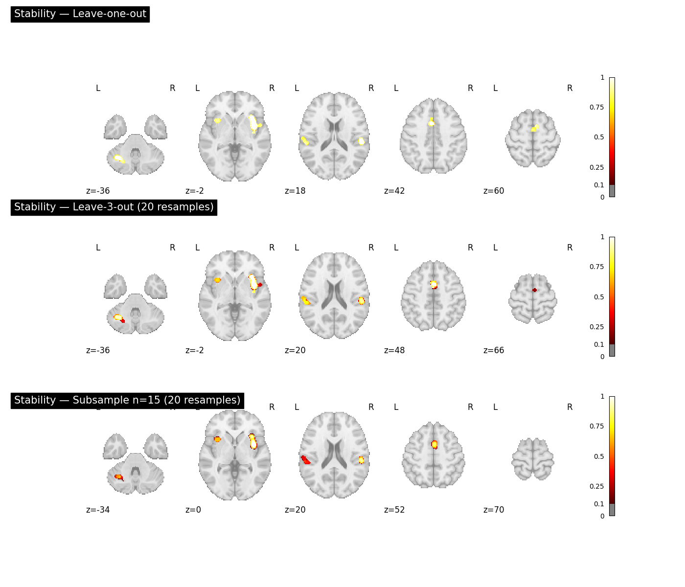
Stability maps: three policies side by side
All three policies yield a voxelwise stability map on the same 0–1 scale. Comparing them reveals whether spatial reliability is preserved as the perturbation grows stronger (leave-1-out → leave-3-out → subsample 75 %). Voxels that remain stable across all three policies are the most trustworthy.
stability_key = f"{TARGET_IMAGE}_diag-ResampledStability"
configs = [
    (result_loo, "Leave-one-out"),
    (result_lko, f"Leave-{rs_lko.k}-out ({N_RESAMPLES} resamples)"),
    (result_sub, f"Subsample n={target_n} ({N_RESAMPLES} resamples)"),
]

fig, axes = plt.subplots(len(configs), 1, figsize=(14, 4 * len(configs)))
for ax, (res, title) in zip(axes, configs):
    plot_stat_map(
        res.get_map(stability_key),
        cut_coords=5,
        display_mode="z",
        title=f"Stability — {title}",
        threshold=0.1,
        vmin=0,
        vmax=1,
        cmap="hot",
        symmetric_cbar=False,
        axes=ax,
        figure=fig,
    )
fig.tight_layout()
plt.show()
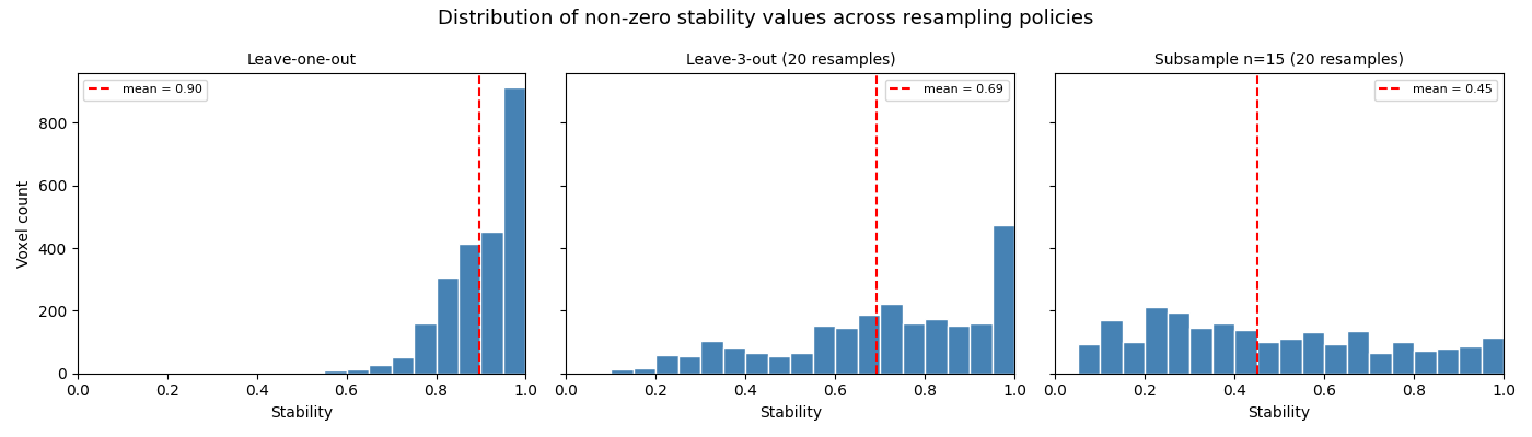
Distribution of stability values
Plotting the distribution of non-zero stability values across all three policies shows how the overall robustness of the result changes as the perturbation grows. A distribution concentrated near 1 indicates a stable result; a broad or left-skewed distribution signals spatial fragility.
fig, axes = plt.subplots(1, len(configs), figsize=(14, 4), sharey=True)
for ax, (res, title) in zip(axes, configs):
    stab = res.get_map(stability_key, return_type="array")
    nonzero = stab[stab > 0]
    ax.hist(nonzero, bins=20, range=(0, 1), color="steelblue", edgecolor="white")
    ax.set_title(title, fontsize=10)
    ax.set_xlabel("Stability")
    ax.set_xlim(0, 1)
    mean_val = nonzero.mean() if len(nonzero) > 0 else 0
    ax.axvline(mean_val, color="red", linestyle="--", label=f"mean = {mean_val:.2f}")
    ax.legend(fontsize=8)
axes[0].set_ylabel("Voxel count")
fig.suptitle("Distribution of non-zero stability values across resampling policies", fontsize=13)
fig.tight_layout()
plt.show()
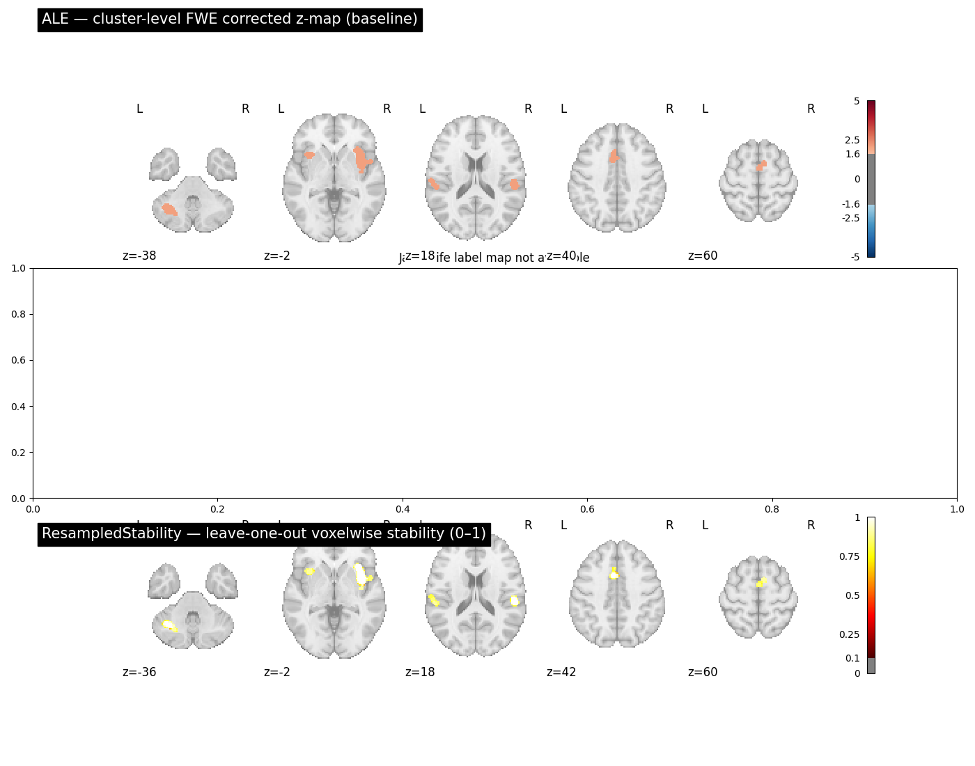
Baseline, Jackknife clusters, and stability side by side
Placing the corrected z-map, the Jackknife cluster-label map, and the leave-one-out stability map on the same axial slices makes it easy to see whether the regions identified as clusters are also the regions with the highest voxelwise stability. When they agree, the result is doubly supported. When the stability map is patchy or low inside a cluster boundary, that cluster deserves more scrutiny.
fig, axes = plt.subplots(3, 1, figsize=(14, 11))

plot_stat_map(
    result.get_map(TARGET_IMAGE),
    cut_coords=5,
    display_mode="z",
    title="ALE — cluster-level FWE corrected z-map (baseline)",
    threshold=1.65,
    cmap="RdBu_r",
    symmetric_cbar=True,
    vmax=5,
    axes=axes[0],
    figure=fig,
)

if contrib_df is not None and not contrib_df.empty:
    label_key = f"label_{TARGET_IMAGE}_tail-positive"
    if label_key in result_jk.maps:
        plot_stat_map(
            result_jk.get_map(label_key),
            cut_coords=5,
            display_mode="z",
            title="Jackknife — cluster label map (colour = cluster ID)",
            threshold=0.5,
            cmap="Set1",
            symmetric_cbar=False,
            axes=axes[1],
            figure=fig,
        )
    else:
        axes[1].set_title("Jackknife label map not available")
else:
    axes[1].set_title("No clusters found for Jackknife")

plot_stat_map(
    result_loo.get_map(stability_key),
    cut_coords=5,
    display_mode="z",
    title="ResampledStability — leave-one-out voxelwise stability (0–1)",
    threshold=0.1,
    vmin=0,
    vmax=1,
    cmap="hot",
    symmetric_cbar=False,
    axes=axes[2],
    figure=fig,
)

fig.tight_layout()
plt.show()
Numerical stability summary across policies
The table below shows how many voxels survive at three stability thresholds (> 0, ≥ 0.5, ≥ 0.8) under each resampling policy. A strict threshold of 0.8 retains only the voxels that survived thresholding in at least 80 % of resamples — a reasonable bar for high-confidence reporting.
rows = []
for res, label in configs:
    stab = res.get_map(stability_key, return_type="array")
    nonzero = stab[stab > 0]
    rows.append(
        {
            "Policy": label,
            "N replicates": int(
                res.tables[f"{TARGET_IMAGE}_diag-ResampledStability_tab-summary"][
                    "n_resamples"
                ].iloc[0]
            ),
            "Stable voxels (>0)": int(len(nonzero)),
            "Stable voxels (≥0.5)": int((stab >= 0.5).sum()),
            "Stable voxels (≥0.8)": int((stab >= 0.8).sum()),
            "Mean stability (nonzero)": (
                round(float(nonzero.mean()), 3) if len(nonzero) > 0 else 0.0
            ),
        }
    )

pd.DataFrame(rows).set_index("Policy")
Key differences at a glance
Feature |
Jackknife |
ResampledStability |
|---|---|---|
Question answered |
Which studies drive each cluster? |
How reliably does each voxel survive thresholding? |
Output granularity |
Study × cluster (one scalar per pair) |
Voxelwise map (one value per brain voxel) |
Output range |
0–1 (proportional contribution) |
0–1 (proportion of resamples surviving threshold) |
Number of estimator refits |
N (one per study) |
|
Resampling policy |
Fixed: leave-one-out |
Choice: leave_1_out / leave_k_out / subsample |
Works with pairwise estimators? |
Yes (v 0.1.2+) |
No |
Null distribution rebuilt per replicate? |
No (fast path for CBMA) |
Depends on policy (subsample rebuilds it) |
Typical compute cost |
O(N) estimator fits |
O(n_resamples) estimator fits |
Default in CBMAWorkflow / IBMAWorkflow? |
Yes |
No |
Primary use case |
Influence and outlier detection |
Spatial reliability for publication figures |
When to use Jackknife
Use Jackknife whenever you want to know which
studies are responsible for a significant cluster. It is the right first
diagnostic in almost every meta-analysis:
It is fast — N refits where N is the study count, without rebuilding the null distribution.
It is interpretable — reviewers can cross-check high-contribution studies against the original publications.
It works with all single-sample and pairwise estimators in NiMARE.
It runs automatically inside
CBMAWorkflowandIBMAWorkflow.
If any study shows a contribution > 0.8 in a cluster, inspect it carefully: unusual coordinate densities, atypical sample sizes, or duplicate peaks from the same laboratory are common culprits.
When to use ResampledStability
Use ResampledStability when you need a
spatially explicit reliability map — for example to include in a
supplementary figure, to compare the robustness of two estimators, or to
flag voxels at the edges of clusters that may not be trustworthy.
Choose
"leave_1_out"for small datasets (< 25 studies) where each study carries substantial weight.Choose
"leave_k_out"for larger datasets (> 30 studies).Choose
"subsample"for larger datasets (> 30 studies) or when you want to quantify what fraction of the result survives at a reduced sample size (e.g.target_n = int(0.75 * n_studies)).
A practical benchmark: report mean stability per cluster; flag clusters with
mean stability < 0.5 under "leave_1_out" as potentially unreliable even
if they survived FWE correction.
Recommended workflow
Run
Jackknife(or useCBMAWorkflowwhich runs it automatically) to identify influential studies.For publication, add
ResampledStabilitywith"leave_1_out"(small datasets) or"subsample"(large datasets) and include the stability map as a supplementary figure.Interpret the two diagnostics together: a cluster that is both driven by a single study (high Jackknife contribution) and spatially unstable (low ResampledStability) should be downgraded in confidence or omitted.
References
Total running time of the script: (0 minutes 23.384 seconds)