Predictive ALE: fast FWE correction without Monte Carlo

Standard ALE family-wise error (FWE) correction uses Monte Carlo permutations to build a null distribution of maximum ALE statistics. For large datasets this can take hours.

Predictive ALE [1] replaces the Monte Carlo step with a pair of pre-trained XGBoost regressors that predict the voxel-level and cluster-level FWE thresholds directly from three study-level metadata quantities:

• number of experiments (n_experiments),

• per-experiment participant count (n_subjects),

• per-experiment focus count (n_foci).

The regressors were fitted on a large grid of simulated ALE datasets and are packaged with NiMARE. Applying them takes milliseconds.

In-sample vs. out-of-sample

The models are valid only for datasets whose metadata falls within the training range used to fit the regressors. Datasets that fall inside this range are called in-sample; datasets whose metadata exceeds the limits are out-of-sample and will raise a PredictiveCutoffError.

In-sample requirements:

Feature	Min	Max
n_experiments	1	150
subjects/experiment	1	300
foci/experiment	0	150

In this example we:

1. Build a simulated in-sample dataset and verify that predictive ALE succeeds.

2. Show the predicted thresholds and resulting maps.

3. Compare predictive FWE to Monte Carlo FWE on the same data.

4. Build a simulated out-of-sample dataset (too many subjects), observe the error, and demonstrate the appropriate Monte Carlo fallback.

Note

Predictive FWE requires the optional xgboost dependency:

pip install nimare[predictive]

Simulated in-sample dataset

create_coordinate_studyset() generates a synthetic coordinate dataset. Sample size is stored in the studyset metadata and is automatically picked up by ALE when it fits the data.

Dataset characteristics:

• 20 experiments

• 25 participants per experiment (≤ 300 → in-sample)

• 1 ground-truth focus + 2 random noise foci per experiment (3 foci total, ≤ 150 → in-sample)

• 80 % of studies contain the ground-truth focus

Note

For real analyses, use at least n_iters=5000 for Monte Carlo corrections. We use 100 iterations here only for documentation-build speed.

import warnings
from pprint import pprint

import matplotlib.pyplot as plt
import numpy as np
from nilearn.plotting import plot_stat_map

from nimare.generate import create_coordinate_studyset
from nimare.meta.cbma.ale import ALE

N_ITERS = 100  # use 5000 for real analyses

ground_truth_foci, studyset_in = create_coordinate_studyset(
    foci=1,
    foci_percentage="80%",
    fwhm=10,
    sample_size=25,
    n_studies=20,
    n_noise_foci=2,
    seed=42,
)

print(f"Ground-truth focus (mm): {ground_truth_foci}")
print(f"Studies: {len(studyset_in.study_ids)}")

Ground-truth focus (mm): [(np.float64(4.0), np.float64(-2.0), np.float64(24.0))]
Studies: 20

Inspect dataset metadata features used by predictive ALE

_predictive_counts() extracts the per-experiment counts used by the packaged regressors. Printing them before correction confirms the dataset is in-sample.

ale_in = ALE()
result_in = ale_in.fit(studyset_in)

# _predictive_counts extracts the per-experiment subject and focus counts from
# the fitted estimator inputs.
nexp, nsub, nfoci = ale_in._predictive_counts()

print(f"n_experiments : {nexp}  (limit ≤ 150)")
print(f"subjects/exp  : min={nsub.min():.0f}, max={nsub.max():.0f}  (limit ≤ 300)")
print(f"foci/exp      : min={nfoci.min():.0f}, max={nfoci.max():.0f}  (limit ≤ 150)")
print("→ All three features are within the in-sample range.")

n_experiments : 20  (limit ≤ 150)
subjects/exp  : min=25, max=25  (limit ≤ 300)
foci/exp      : min=2, max=3  (limit ≤ 150)
→ All three features are within the in-sample range.

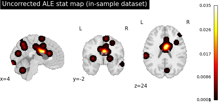
Fit ALE and inspect the uncorrected stat map

Before applying any correction we look at the raw ALE convergence map.

stat_img = result_in.get_map("stat")

plot_stat_map(
    stat_img,
    cut_coords=ground_truth_foci[0],
    draw_cross=False,
    cmap="hot",
    symmetric_cbar=False,
    threshold=0.0001,
    title="Uncorrected ALE stat map (in-sample dataset)",
)

<nilearn.plotting.displays._slicers.OrthoSlicer object at 0x784a8c9ebac0>

Predictive FWE correction (in-sample)

FWECorrector with method='predictive' calls the packaged XGBoost regressors. This takes milliseconds and produces both a voxel-level FWE map and a cluster-level FWE map.

from nimare.correct import FWECorrector
from nimare.meta.cbma.predictive import predict_cutoffs

cutoffs = predict_cutoffs(nexp, nsub, nfoci)
print(f"Predicted voxel-level FWE threshold (ALE stat) : {cutoffs['vfwe']:.6f}")
print(f"Predicted cluster-size FWE threshold (voxels)  : {cutoffs['cfwe']}")

corr_pred = FWECorrector(method="predictive")
cres_pred = corr_pred.transform(result_in)

print("Available predictive-FWE maps:")
pprint([k for k in cres_pred.maps if "predictive" in k])

/home/docs/checkouts/readthedocs.org/user_builds/nimare/checkouts/latest/nimare/meta/cbma/predictive.py:29: RuntimeWarning: Precision loss occurred in moment calculation due to catastrophic cancellation. This occurs when the data are nearly identical. Results may be unreliable.
  value = func(values)
Predicted voxel-level FWE threshold (ALE stat) : 0.016512
Predicted cluster-size FWE threshold (voxels)  : 91
/home/docs/checkouts/readthedocs.org/user_builds/nimare/checkouts/latest/nimare/meta/cbma/predictive.py:29: RuntimeWarning: Precision loss occurred in moment calculation due to catastrophic cancellation. This occurs when the data are nearly identical. Results may be unreliable.
  value = func(values)
Available predictive-FWE maps:
['p_level-voxel_corr-FWE_method-predictive',
 'z_level-voxel_corr-FWE_method-predictive',
 'logp_level-voxel_corr-FWE_method-predictive',
 'p_desc-size_level-cluster_corr-FWE_method-predictive',
 'z_desc-size_level-cluster_corr-FWE_method-predictive',
 'logp_desc-size_level-cluster_corr-FWE_method-predictive']

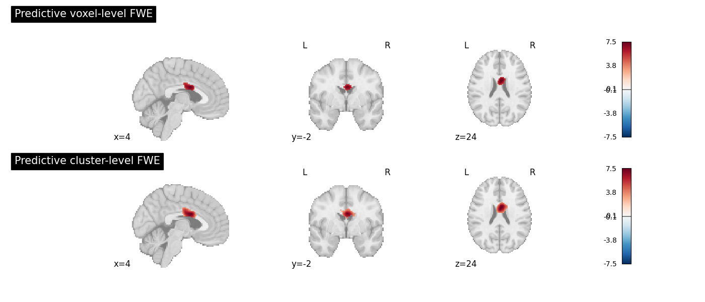
Visualize the predictive FWE maps

Two maps are produced:

• Voxel-level FWE (z_level-voxel_corr-FWE_method-predictive): voxels whose ALE statistic exceeds the predicted vFWE threshold.

• Cluster-level FWE (z_desc-size_level-cluster_corr-FWE_method-predictive): voxels belonging to clusters whose size exceeds the predicted cFWE threshold.

fig, axes = plt.subplots(figsize=(14, 6), nrows=2)

plot_stat_map(
    cres_pred.get_map("z_level-voxel_corr-FWE_method-predictive"),
    cut_coords=ground_truth_foci[0],
    draw_cross=False,
    cmap="RdBu_r",
    symmetric_cbar=True,
    threshold=0.1,
    title="Predictive voxel-level FWE",
    axes=axes[0],
    figure=fig,
)

plot_stat_map(
    cres_pred.get_map("z_desc-size_level-cluster_corr-FWE_method-predictive"),
    cut_coords=ground_truth_foci[0],
    draw_cross=False,
    cmap="RdBu_r",
    symmetric_cbar=True,
    threshold=0.1,
    title="Predictive cluster-level FWE",
    axes=axes[1],
    figure=fig,
)

fig.tight_layout()
fig.show()

/home/docs/checkouts/readthedocs.org/user_builds/nimare/checkouts/latest/examples/02_meta-analyses/15_plot_predictive_ale.py:193: UserWarning: This figure includes Axes that are not compatible with tight_layout, so results might be incorrect.
  fig.tight_layout()

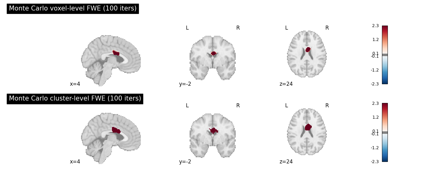
Comparison: predictive FWE vs. Monte Carlo FWE

Running Monte Carlo FWE on the same dataset lets us see how closely the predicted thresholds match the permutation-based ones.

Note

The Monte Carlo result with n_iters=100 is noisy. Use 5000 or more iterations for publication-quality comparisons. The Monte Carlo threshold estimates stabilize as n_iters grows.

corr_mc = FWECorrector(method="montecarlo", n_iters=N_ITERS, n_cores=1)
cres_mc = corr_mc.transform(result_in)

# The Monte Carlo voxel-level null stores the per-iteration maximum ALE stat.
mc_null = cres_mc.estimator.null_distributions_.get(
    "values_level-voxel_corr-fwe_method-montecarlo", np.array([])
)
mc_vfwe_thresh = float(np.percentile(mc_null, 95)) if mc_null.size else float("nan")
mc_cfwe_thresh = float(
    np.percentile(
        cres_mc.estimator.null_distributions_.get(
            "values_desc-size_level-cluster_corr-fwe_method-montecarlo", [np.nan]
        ),
        95,
    )
)

print("Threshold comparison:")
print(f"  Predictive vFWE  : {cutoffs['vfwe']:.6f}")
print(f"  Monte Carlo vFWE : {mc_vfwe_thresh:.6f}  ({N_ITERS} iters)")
print(f"  Predictive cFWE  : {cutoffs['cfwe']} voxels")
print(f"  Monte Carlo cFWE : {mc_cfwe_thresh:.1f} voxels  ({N_ITERS} iters)")

fig2, axes2 = plt.subplots(figsize=(14, 6), nrows=2)

plot_stat_map(
    cres_mc.get_map("z_level-voxel_corr-FWE_method-montecarlo"),
    cut_coords=ground_truth_foci[0],
    draw_cross=False,
    cmap="RdBu_r",
    symmetric_cbar=True,
    threshold=0.1,
    title=f"Monte Carlo voxel-level FWE ({N_ITERS} iters)",
    axes=axes2[0],
    figure=fig2,
)

plot_stat_map(
    cres_mc.get_map("z_desc-size_level-cluster_corr-FWE_method-montecarlo"),
    cut_coords=ground_truth_foci[0],
    draw_cross=False,
    cmap="RdBu_r",
    symmetric_cbar=True,
    threshold=0.1,
    title=f"Monte Carlo cluster-level FWE ({N_ITERS} iters)",
    axes=axes2[1],
    figure=fig2,
)

fig2.tight_layout()
fig2.show()

  0%|          | 0/100 [00:00<?, ?it/s]
  4%|▍         | 4/100 [00:00<00:02, 38.05it/s]
  8%|▊         | 8/100 [00:00<00:02, 38.10it/s]
 12%|█▏        | 12/100 [00:00<00:02, 38.31it/s]
 16%|█▌        | 16/100 [00:00<00:02, 38.28it/s]
 20%|██        | 20/100 [00:00<00:02, 38.32it/s]
 24%|██▍       | 24/100 [00:00<00:01, 38.23it/s]
 28%|██▊       | 28/100 [00:00<00:01, 38.40it/s]
 32%|███▏      | 32/100 [00:00<00:01, 38.59it/s]
 36%|███▌      | 36/100 [00:00<00:01, 38.76it/s]
 40%|████      | 40/100 [00:01<00:01, 38.74it/s]
 44%|████▍     | 44/100 [00:01<00:01, 38.78it/s]
 48%|████▊     | 48/100 [00:01<00:01, 38.78it/s]
 52%|█████▏    | 52/100 [00:01<00:01, 38.74it/s]
 56%|█████▌    | 56/100 [00:01<00:01, 38.73it/s]
 60%|██████    | 60/100 [00:01<00:01, 38.47it/s]
 64%|██████▍   | 64/100 [00:01<00:00, 38.55it/s]
 68%|██████▊   | 68/100 [00:01<00:00, 38.11it/s]
 72%|███████▏  | 72/100 [00:01<00:00, 38.12it/s]
 76%|███████▌  | 76/100 [00:01<00:00, 38.31it/s]
 80%|████████  | 80/100 [00:02<00:00, 38.40it/s]
 84%|████████▍ | 84/100 [00:02<00:00, 38.41it/s]
 88%|████████▊ | 88/100 [00:02<00:00, 38.44it/s]
 92%|█████████▏| 92/100 [00:02<00:00, 38.41it/s]
 96%|█████████▌| 96/100 [00:02<00:00, 38.53it/s]
100%|██████████| 100/100 [00:02<00:00, 38.38it/s]
100%|██████████| 100/100 [00:02<00:00, 38.45it/s]
Threshold comparison:
  Predictive vFWE  : 0.016512
  Monte Carlo vFWE : 0.017048  (100 iters)
  Predictive cFWE  : 91 voxels
  Monte Carlo cFWE : 91.2 voxels  (100 iters)
/home/docs/checkouts/readthedocs.org/user_builds/nimare/checkouts/latest/examples/02_meta-analyses/15_plot_predictive_ale.py:255: UserWarning: This figure includes Axes that are not compatible with tight_layout, so results might be incorrect.
  fig2.tight_layout()

Simulated out-of-sample dataset

A dataset with sample_size=350 violates the max subjects ≤ 300 requirement. Calling transform() raises a PredictiveCutoffError because the XGBoost models were not trained on data in that range.

Other out-of-sample conditions:

• More than 150 experiments (n_studies > 150)

• More than 150 foci per experiment (n_noise_foci > 149)

from nimare.meta.cbma.predictive import PredictiveCutoffError

_, studyset_out = create_coordinate_studyset(
    foci=1,
    foci_percentage="80%",
    fwhm=10,
    sample_size=350,    # ← exceeds the 300-subject limit
    n_studies=20,
    n_noise_foci=2,
    seed=42,
)

ale_out = ALE()
result_out = ale_out.fit(studyset_out)

nexp_out, nsub_out, nfoci_out = ale_out._predictive_counts()
print(f"n_experiments : {nexp_out}  (limit ≤ 150)")
print(f"subjects/exp  : min={nsub_out.min():.0f}, max={nsub_out.max():.0f}  (limit ≤ 300)")
print(f"foci/exp      : min={nfoci_out.min():.0f}, max={nfoci_out.max():.0f}  (limit ≤ 150)")
print("→ max subjects/exp EXCEEDS the in-sample limit.")

try:
    corr_pred_out = FWECorrector(method="predictive")
    cres_pred_out = corr_pred_out.transform(result_out)
except PredictiveCutoffError as exc:
    print(f"\nPredictiveCutoffError raised as expected:\n  {exc}")

n_experiments : 20  (limit ≤ 150)
subjects/exp  : min=350, max=350  (limit ≤ 300)
foci/exp      : min=2, max=3  (limit ≤ 150)
→ max subjects/exp EXCEEDS the in-sample limit.

PredictiveCutoffError raised as expected:
  Predictive cutoff is out of the packaged model's supported range: max subjects per experiment (350) exceeds 300.

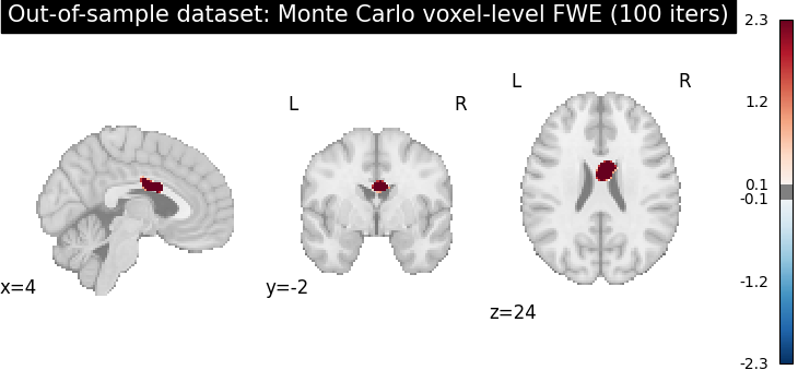
Fallback: Monte Carlo FWE for out-of-sample datasets

When a dataset is out-of-sample for predictive ALE, Monte Carlo FWE is the appropriate alternative. It always works regardless of dataset size, though it is slower.

print("Falling back to Monte Carlo FWE for the out-of-sample dataset...")
with warnings.catch_warnings():
    warnings.simplefilter("ignore")
    corr_mc_out = FWECorrector(method="montecarlo", n_iters=N_ITERS, n_cores=1)
    cres_mc_out = corr_mc_out.transform(result_out)

plot_stat_map(
    cres_mc_out.get_map("z_level-voxel_corr-FWE_method-montecarlo"),
    cut_coords=ground_truth_foci[0],
    draw_cross=False,
    cmap="RdBu_r",
    symmetric_cbar=True,
    threshold=0.1,
    title=f"Out-of-sample dataset: Monte Carlo voxel-level FWE ({N_ITERS} iters)",
)

Falling back to Monte Carlo FWE for the out-of-sample dataset...

  0%|          | 0/100 [00:00<?, ?it/s]
  5%|▌         | 5/100 [00:00<00:02, 41.84it/s]
 10%|█         | 10/100 [00:00<00:02, 41.87it/s]
 15%|█▌        | 15/100 [00:00<00:02, 41.73it/s]
 20%|██        | 20/100 [00:00<00:01, 41.66it/s]
 25%|██▌       | 25/100 [00:00<00:01, 41.61it/s]
 30%|███       | 30/100 [00:00<00:01, 41.70it/s]
 35%|███▌      | 35/100 [00:00<00:01, 41.75it/s]
 40%|████      | 40/100 [00:00<00:01, 41.75it/s]
 45%|████▌     | 45/100 [00:01<00:01, 41.81it/s]
 50%|█████     | 50/100 [00:01<00:01, 41.72it/s]
 55%|█████▌    | 55/100 [00:01<00:01, 41.57it/s]
 60%|██████    | 60/100 [00:01<00:00, 41.34it/s]
 65%|██████▌   | 65/100 [00:01<00:00, 41.31it/s]
 70%|███████   | 70/100 [00:01<00:00, 41.45it/s]
 75%|███████▌  | 75/100 [00:01<00:00, 41.54it/s]
 80%|████████  | 80/100 [00:01<00:00, 41.56it/s]
 85%|████████▌ | 85/100 [00:02<00:00, 41.69it/s]
 90%|█████████ | 90/100 [00:02<00:00, 41.78it/s]
 95%|█████████▌| 95/100 [00:02<00:00, 41.71it/s]
100%|██████████| 100/100 [00:02<00:00, 41.72it/s]
100%|██████████| 100/100 [00:02<00:00, 41.64it/s]

<nilearn.plotting.displays._slicers.OrthoSlicer object at 0x784a923f78b0>

Summary: when to use predictive vs. Monte Carlo FWE

Criterion	Predictive FWE	Monte Carlo FWE
Speed	Milliseconds	Minutes to hours
Requires xgboost	Yes	No
Requires sample_size metadata	Yes	No
n_experiments limit	≤ 150	No limit
max subjects/experiment limit	≤ 300	No limit
max foci/experiment limit	≤ 150	No limit
Produces cluster-level FWE	Yes	Yes
Appropriate for out-of-sample data	No (raises error)	Yes

Recommended workflow

1. Check whether your dataset is in-sample using _predictive_counts().

2. If in-sample, apply FWECorrector(method='predictive') for fast thresholding.

3. If out-of-sample, fall back to FWECorrector(method='montecarlo').

Boilerplate text and references

print("Predictive-FWE result description:")
pprint(cres_pred.description_)

Predictive-FWE result description:
('An activation likelihood estimation (ALE) meta-analysis '
 '\\citep{turkeltaub2002meta,turkeltaub2012minimizing,eickhoff2012activation} '
 'was performed with NiMARE 0.20.0+2.gba8d921 (RRID:SCR_017398; '
 '\\citealt{Salo2023}), using a(n) ALE kernel. An ALE kernel '
 '\\citep{eickhoff2012activation} was used to generate study-wise modeled '
 'activation maps from coordinates. In this kernel method, each coordinate is '
 'convolved with a Gaussian kernel with full-width at half max values '
 'determined on a study-wise basis based on the study sample sizes according '
 'to the formulae provided in \\cite{eickhoff2012activation}. For voxels with '
 'overlapping kernels, the maximum value was retained. ALE values were '
 'converted to p-values using an approximate null distribution '
 '\\citep{eickhoff2012activation}. The input dataset included 56 foci from 20 '
 'experiments, with a total of 500 participants. Family-wise error correction '
 'was approximated with predictive ALE cutoffs. Voxel-level and cluster-size '
 'thresholds were predicted from experiment-level subject and focus counts '
 'using packaged XGBoost regressors trained on simulated ALE datasets, as '
 'described in :footcite:t:`10.1162/imag_a_00423`.')

References

[1]

Lennart Frahm, Kaustubh R. Patil, Theodore D. Satterthwaite, Peter T. Fox, Simon B. Eickhoff, and Robert Langner. Predictive modeling of significance thresholding in activation likelihood estimation meta-analysis. Imaging Neuroscience, 3:imag_a_00423, 01 2025. URL: https://doi.org/10.1162/imag_a_00423, arXiv:https://direct.mit.edu/imag/article-pdf/doi/10.1162/imag_a_00423/2483917/imag_a_00423.pdf, doi:10.1162/imag_a_00423.