Comparing ALE-based pairwise contrast strategies

When comparing two groups of neuroimaging studies, NiMARE offers three complementary approaches:

• ALESubtraction — two-sided, whole-mask subtraction with a permutation null.

• ContrastWorkflow — main-effect-gated subtraction that mirrors the original GingerALE-style logic [1].

• BalancedALESubtraction — balanced subsampling subtraction that corrects for unequal group sizes [2].

All three use the ALE modelled-activation framework, but they differ in how group sizes are handled, whether main-effect information gates directional inference, and what output maps are returned.

ALESubtraction (standalone): evaluates the group difference (Group 1 − Group 2) in a two-sided manner across all voxels in the analysis mask simultaneously, without any prior information about where each group shows a reliable main effect. Groups are compared at their natural sizes; no resampling is performed. A corrector is applied as a separate step after fitting.

ContrastWorkflow: implements GingerALE-style main-effect-gated approach [1]. It first computes and corrects a within-group ALE for each group, thresholds those corrected maps at a chosen α, and then passes the surviving voxels as directional inference masks to ALESubtraction. Group 1 > Group 2 differences are evaluated only where Group 1 shows a surviving main effect, and Group 2 > Group 1 differences are evaluated only where Group 2 shows a surviving main effect. The workflow also stores the individual main-effect maps and a voxelwise-minimum conjunction map alongside the thresholded contrast. The workflow thresholds the pairwise p-map internally; no additional corrector call is made after the fact.

BalancedALESubtraction: addresses a systematic bias that arises when the two groups contain different numbers of studies [2]. Because ALE values grow with sample size, a naive subtraction will spuriously favour the larger group. This method draws matched-size random subsamples from each group, averages the balanced ALE differences over many draws, and builds a Monte Carlo null from balanced resamples of random foci (or permuted labels). It also produces probabilistic activation maps for each group — the proportion of subsamples in which each voxel survived cluster thresholding — and a conjunction of those probability maps. No separate correction step is needed.

In this example we apply all three approaches to the same two study groups and compare their output maps.

Load data

We use two Sleuth text files bundled with NiMARE that describe pediatric semantic cognition studies [3]. The first group probed semantic world knowledge (e.g., naming an object from its description) and the second group asked children to judge semantic relatedness between words.

Note

For real analyses, use at least n_iters=5000. We use 100 iterations throughout this example purely for documentation-build speed.

import os
from pprint import pprint

import matplotlib.pyplot as plt
from nilearn.plotting import plot_stat_map

from nimare.io import convert_sleuth_to_studyset
from nimare.utils import get_resource_path

N_ITERS = 100

knowledge_file = os.path.join(get_resource_path(), "semantic_knowledge_children.txt")
related_file = os.path.join(get_resource_path(), "semantic_relatedness_children.txt")

knowledge_studyset = convert_sleuth_to_studyset(knowledge_file)
related_studyset = convert_sleuth_to_studyset(related_file)

print(f"Semantic knowledge: {len(knowledge_studyset.studies)} studies")
print(f"Semantic relatedness: {len(related_studyset.studies)} studies")

Semantic knowledge: 21 studies
Semantic relatedness: 16 studies

ALESubtraction (standalone)

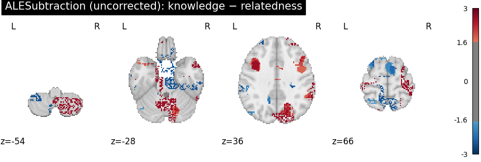
Running ALESubtraction directly compares the two groups across the entire brain mask in a single two-sided permutation test. Positive z-values indicate knowledge > relatedness; negative values indicate relatedness > knowledge.

Unlike the original GingerALE implementation, this NiMARE approach does not restrict testing to regions where either group has a significant main effect, and it does not correct for unequal group sizes. The benefit is a whole-mask search without main-effect gating; the trade-off is that it may detect differences in regions where neither group shows a reliable main effect, and results can be skewed when group sizes differ substantially.

After fitting, a FWECorrector (or FDR) can be applied to the returned MetaResult in the usual way.

from nimare.meta.cbma.ale import ALESubtraction

subtraction = ALESubtraction(n_iters=N_ITERS, n_cores=1)
subtraction_result = subtraction.fit(knowledge_studyset, related_studyset)

print("ALESubtraction uncorrected output maps:")
pprint(list(subtraction_result.maps.keys()))

  0%|          | 0/100 [00:00<?, ?it/s]
  7%|▋         | 7/100 [00:00<00:01, 65.20it/s]
 14%|█▍        | 14/100 [00:00<00:01, 65.02it/s]
 21%|██        | 21/100 [00:00<00:01, 65.13it/s]
 28%|██▊       | 28/100 [00:00<00:01, 64.98it/s]
 35%|███▌      | 35/100 [00:00<00:01, 64.78it/s]
 42%|████▏     | 42/100 [00:00<00:00, 64.89it/s]
 49%|████▉     | 49/100 [00:00<00:00, 64.77it/s]
 56%|█████▌    | 56/100 [00:00<00:00, 64.72it/s]
 63%|██████▎   | 63/100 [00:00<00:00, 64.56it/s]
 70%|███████   | 70/100 [00:01<00:00, 64.39it/s]
 77%|███████▋  | 77/100 [00:01<00:00, 64.36it/s]
 84%|████████▍ | 84/100 [00:01<00:00, 64.46it/s]
 91%|█████████ | 91/100 [00:01<00:00, 64.71it/s]
 98%|█████████▊| 98/100 [00:01<00:00, 64.94it/s]
100%|██████████| 100/100 [00:01<00:00, 64.78it/s]
ALESubtraction uncorrected output maps:
['stat_desc-group1MinusGroup2',
 'p_desc-group1MinusGroup2',
 'z_desc-group1MinusGroup2',
 'logp_desc-group1MinusGroup2',
 'stat_desc-group1',
 'p_desc-group1',
 'z_desc-group1',
 'logp_desc-group1',
 'stat_desc-group2',
 'p_desc-group2',
 'z_desc-group2',
 'logp_desc-group2']

Visualize the uncorrected subtraction z-map.

plot_stat_map(
    subtraction_result.get_map("z_desc-group1MinusGroup2"),
    cut_coords=4,
    display_mode="z",
    title="ALESubtraction (uncorrected): knowledge − relatedness",
    threshold=1.65,
    cmap="RdBu_r",
    symmetric_cbar=True,
    vmax=3,
)

<nilearn.plotting.displays._slicers.ZSlicer object at 0x784a7a82e7b0>

ContrastWorkflow

ContrastWorkflow orchestrates the full main-effect-gated pipeline in a single call:

1. Fit one-sample ALE for Group 1 and correct with the provided corrector (default: FDR with method="indep" and alpha=0.05).

2. Fit one-sample ALE for Group 2 and correct identically.

3. Threshold both corrected maps at alpha to build directional masks.

4. Run ALESubtraction with those masks: Group 1 > Group 2 differences are tested only inside the Group 1 mask; Group 2 > Group 1 differences are tested only inside the Group 2 mask.

5. Threshold the contrast p-map at alpha and store the result.

The returned MetaResult contains all intermediate and final maps. The pairwise p-map is thresholded internally, so no additional corrector call is made after the workflow returns.

ContrastWorkflow accepts a class, an already-initialized instance, or a string (e.g. "alesubtraction") for all three of its main arguments. Passing a class or string lets the workflow propagate n_cores automatically; passing an instance uses whatever settings that instance already carries. Here we pass the class and then lower n_iters on the instantiated estimator to keep the example fast.

from nimare.correct import FDRCorrector
from nimare.workflows.cbma import ContrastWorkflow

contrast_workflow = ContrastWorkflow(
    pairwise_estimator=ALESubtraction,
    corrector=FDRCorrector(method="indep", alpha=0.05),
    alpha=0.05,
    n_cores=1,
)
contrast_workflow.pairwise_estimator.n_iters = N_ITERS
contrast_result = contrast_workflow.fit(knowledge_studyset, related_studyset)

print("ContrastWorkflow output maps:")
pprint(list(contrast_result.maps.keys()))

  0%|          | 0/100 [00:00<?, ?it/s]
  7%|▋         | 7/100 [00:00<00:01, 65.98it/s]
 14%|█▍        | 14/100 [00:00<00:01, 65.94it/s]
 21%|██        | 21/100 [00:00<00:01, 66.62it/s]
 28%|██▊       | 28/100 [00:00<00:01, 65.91it/s]
 35%|███▌      | 35/100 [00:00<00:00, 66.14it/s]
 42%|████▏     | 42/100 [00:00<00:00, 66.37it/s]
 49%|████▉     | 49/100 [00:00<00:00, 66.64it/s]
 56%|█████▌    | 56/100 [00:00<00:00, 66.92it/s]
 63%|██████▎   | 63/100 [00:00<00:00, 66.64it/s]
 70%|███████   | 70/100 [00:01<00:00, 66.67it/s]
 77%|███████▋  | 77/100 [00:01<00:00, 66.85it/s]
 84%|████████▍ | 84/100 [00:01<00:00, 67.03it/s]
 91%|█████████ | 91/100 [00:01<00:00, 67.03it/s]
 98%|█████████▊| 98/100 [00:01<00:00, 67.17it/s]
100%|██████████| 100/100 [00:01<00:00, 66.73it/s]
ContrastWorkflow output maps:
['stat_desc-group1MinusGroup2',
 'p_desc-group1MinusGroup2',
 'z_desc-group1MinusGroup2',
 'logp_desc-group1MinusGroup2',
 'stat_desc-group1',
 'p_desc-group1',
 'z_desc-group1',
 'logp_desc-group1',
 'stat_desc-group2',
 'p_desc-group2',
 'z_desc-group2',
 'logp_desc-group2',
 'z_desc-group1MainEffect',
 'z_desc-group2MainEffect',
 'z_desc-conjunction',
 'p_desc-contrast',
 'z_desc-contrast',
 'logp_desc-contrast']

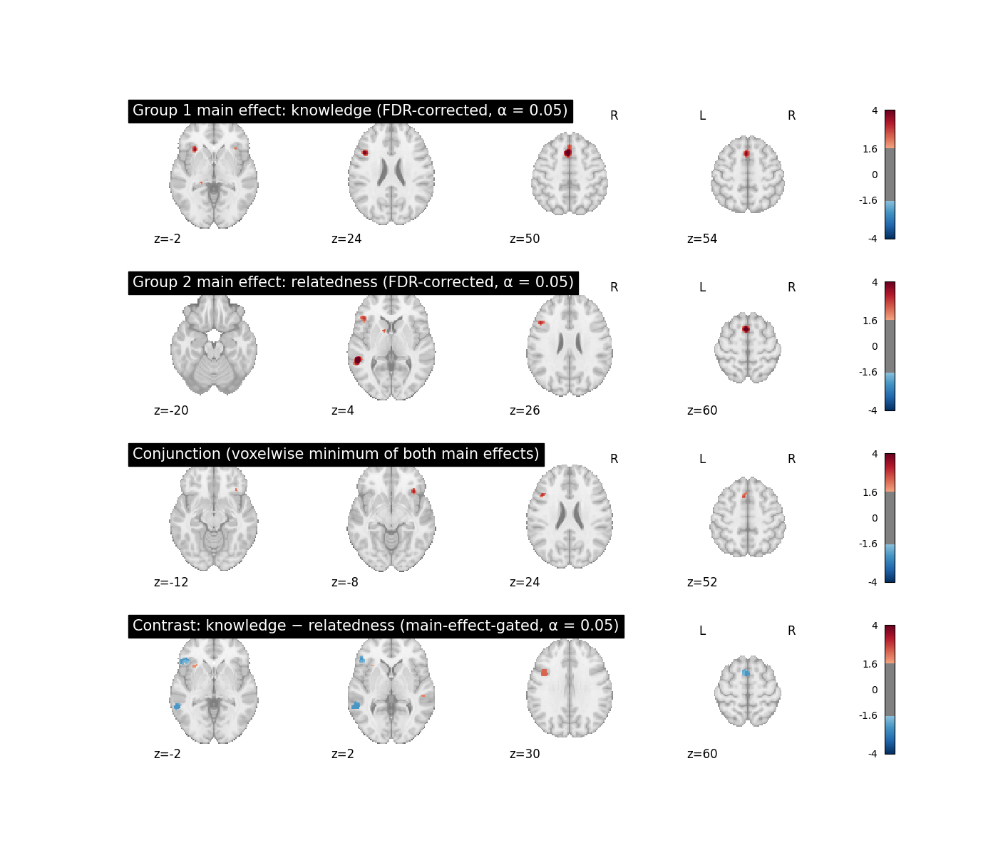
The four key ContrastWorkflow output maps

• z_desc-group1MainEffect — FDR-corrected, thresholded ALE z-map for Group 1 (knowledge). Defines where Group 1 shows reliable activation.

• z_desc-group2MainEffect — same for Group 2 (relatedness).

• z_desc-conjunction — voxelwise minimum of both thresholded main-effect maps; highlights regions where both groups converge.

• z_desc-contrast — the main-effect-gated subtraction contrast, thresholded at alpha. Only voxels that survived in the appropriate main-effect mask contribute to each direction of this map.

fig, axes = plt.subplots(figsize=(14, 12), nrows=4)

plot_stat_map(
    contrast_result.get_map("z_desc-group1MainEffect"),
    cut_coords=4,
    display_mode="z",
    title="Group 1 main effect: knowledge (FDR-corrected, α = 0.05)",
    threshold=1.65,
    cmap="RdBu_r",
    symmetric_cbar=True,
    vmax=4,
    axes=axes[0],
    figure=fig,
)

plot_stat_map(
    contrast_result.get_map("z_desc-group2MainEffect"),
    cut_coords=4,
    display_mode="z",
    title="Group 2 main effect: relatedness (FDR-corrected, α = 0.05)",
    threshold=1.65,
    cmap="RdBu_r",
    symmetric_cbar=True,
    vmax=4,
    axes=axes[1],
    figure=fig,
)

plot_stat_map(
    contrast_result.get_map("z_desc-conjunction"),
    cut_coords=4,
    display_mode="z",
    title="Conjunction (voxelwise minimum of both main effects)",
    threshold=1.65,
    cmap="RdBu_r",
    symmetric_cbar=True,
    vmax=4,
    axes=axes[2],
    figure=fig,
)

plot_stat_map(
    contrast_result.get_map("z_desc-contrast"),
    cut_coords=4,
    display_mode="z",
    title="Contrast: knowledge − relatedness (main-effect-gated, α = 0.05)",
    threshold=1.65,
    cmap="RdBu_r",
    symmetric_cbar=True,
    vmax=4,
    axes=axes[3],
    figure=fig,
)

fig.show()

BalancedALESubtraction

BalancedALESubtraction [2] corrects for a well-known bias: when one group has more studies than the other, ALE values are systematically higher in the larger group, inflating apparent differences. This method avoids that bias through the following steps:

1. Probabilistic activation maps: for each group, many random subsamples of size target_n = min(n₁, n₂) are drawn. Each subsample is meta-analysed with ALE, cluster-thresholded, and each voxel receives a vote (1 if it survived, 0 if not). The resulting probability map is the proportion of subsamples in which a voxel passed the cluster threshold.

2. Mean balanced difference: a separate set of difference_iterations matched-size draw pairs is used to estimate the expected (average) ALE difference under the true group labels.

3. Monte Carlo null: n_iters additional balanced draw pairs are generated under the null (either random-foci or label-permutation) to build an empirical distribution of the minimum and maximum difference, from which two-tailed p-values are derived without any external corrector.

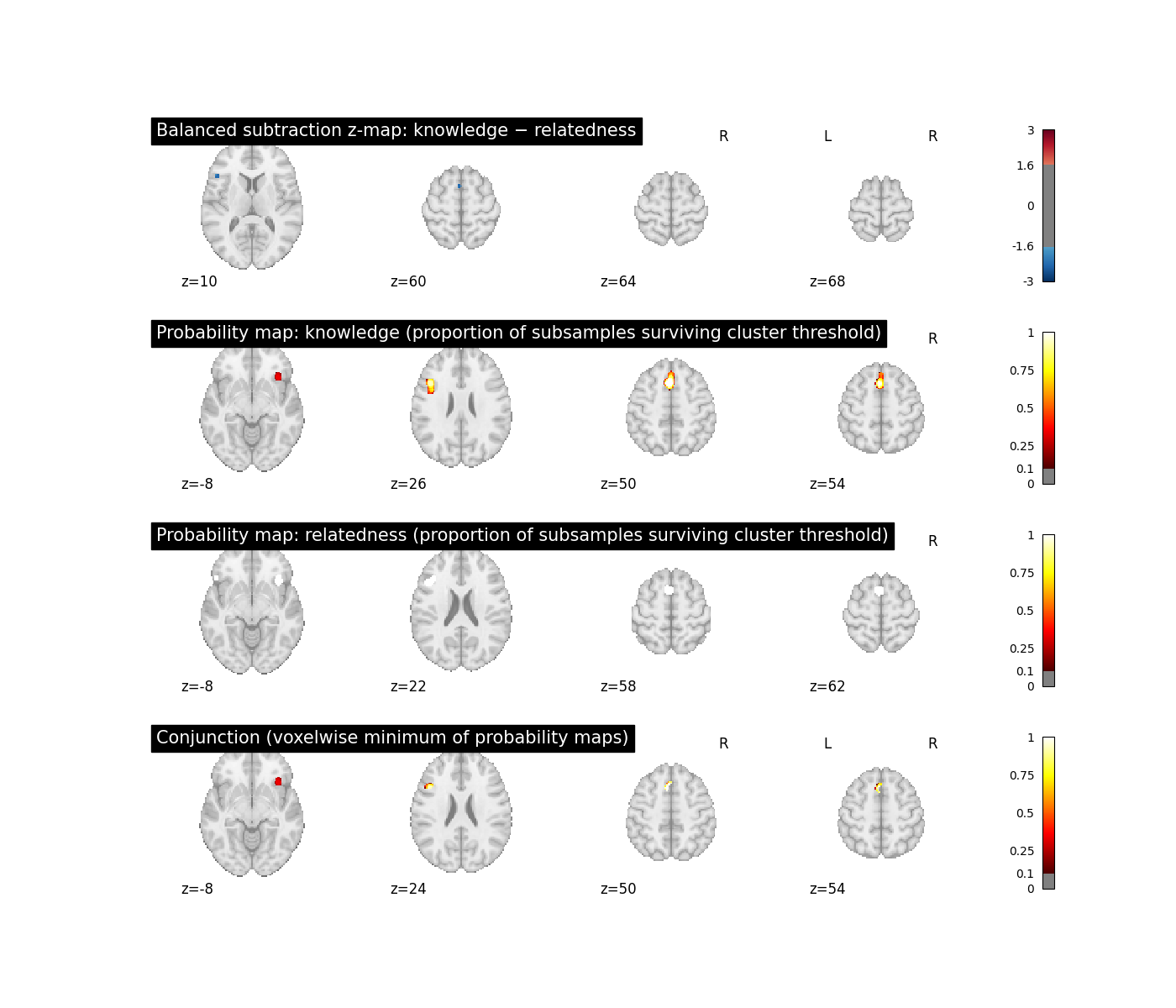
Key outputs:

• z_desc-balancedGroup1MinusGroup2 — z-scored balanced difference map (positive = knowledge > relatedness).

• stat_desc-conjunction — voxelwise minimum of the two probability maps; highlights regions both groups activate consistently across subsamples.

• prob_desc-group1 / prob_desc-group2 — the per-group probability maps.

No separate corrector call is needed; significance thresholding is handled internally via the Monte Carlo extrema.

from nimare.meta.cbma.ale import BalancedALESubtraction

balanced = BalancedALESubtraction(
    n_iters=N_ITERS,
    n_subsamples=100,  # use ≥2500 for real analyses
    difference_iterations=50,  # use ≥1000 for real analyses
    null_method="random-foci",
    n_cores=1,
)
balanced_result = balanced.fit(knowledge_studyset, related_studyset)

print("BalancedALESubtraction output maps:")
pprint(list(balanced_result.maps.keys()))

BalancedALESubtraction output maps:
['stat_desc-balancedGroup1MinusGroup2',
 'p_desc-balancedGroup1MinusGroup2',
 'z_desc-balancedGroup1MinusGroup2',
 'logp_desc-balancedGroup1MinusGroup2',
 'stat_desc-conjunction',
 'prob_desc-group1',
 'prob_desc-group2']

Visualize BalancedALESubtraction outputs.

fig3, axes3 = plt.subplots(figsize=(14, 12), nrows=4)

plot_stat_map(
    balanced_result.get_map("z_desc-balancedGroup1MinusGroup2"),
    cut_coords=4,
    display_mode="z",
    title="Balanced subtraction z-map: knowledge − relatedness",
    threshold=1.65,
    cmap="RdBu_r",
    symmetric_cbar=True,
    vmax=3,
    axes=axes3[0],
    figure=fig3,
)

plot_stat_map(
    balanced_result.get_map("prob_desc-group1"),
    cut_coords=4,
    display_mode="z",
    title="Probability map: knowledge (proportion of subsamples surviving cluster threshold)",
    threshold=0.1,
    cmap="hot",
    symmetric_cbar=False,
    vmax=1,
    axes=axes3[1],
    figure=fig3,
)

plot_stat_map(
    balanced_result.get_map("prob_desc-group2"),
    cut_coords=4,
    display_mode="z",
    title="Probability map: relatedness (proportion of subsamples surviving cluster threshold)",
    threshold=0.1,
    cmap="hot",
    symmetric_cbar=False,
    vmax=1,
    axes=axes3[2],
    figure=fig3,
)

plot_stat_map(
    balanced_result.get_map("stat_desc-conjunction"),
    cut_coords=4,
    display_mode="z",
    title="Conjunction (voxelwise minimum of probability maps)",
    threshold=0.1,
    cmap="hot",
    symmetric_cbar=False,
    vmax=1,
    axes=axes3[3],
    figure=fig3,
)

fig3.show()

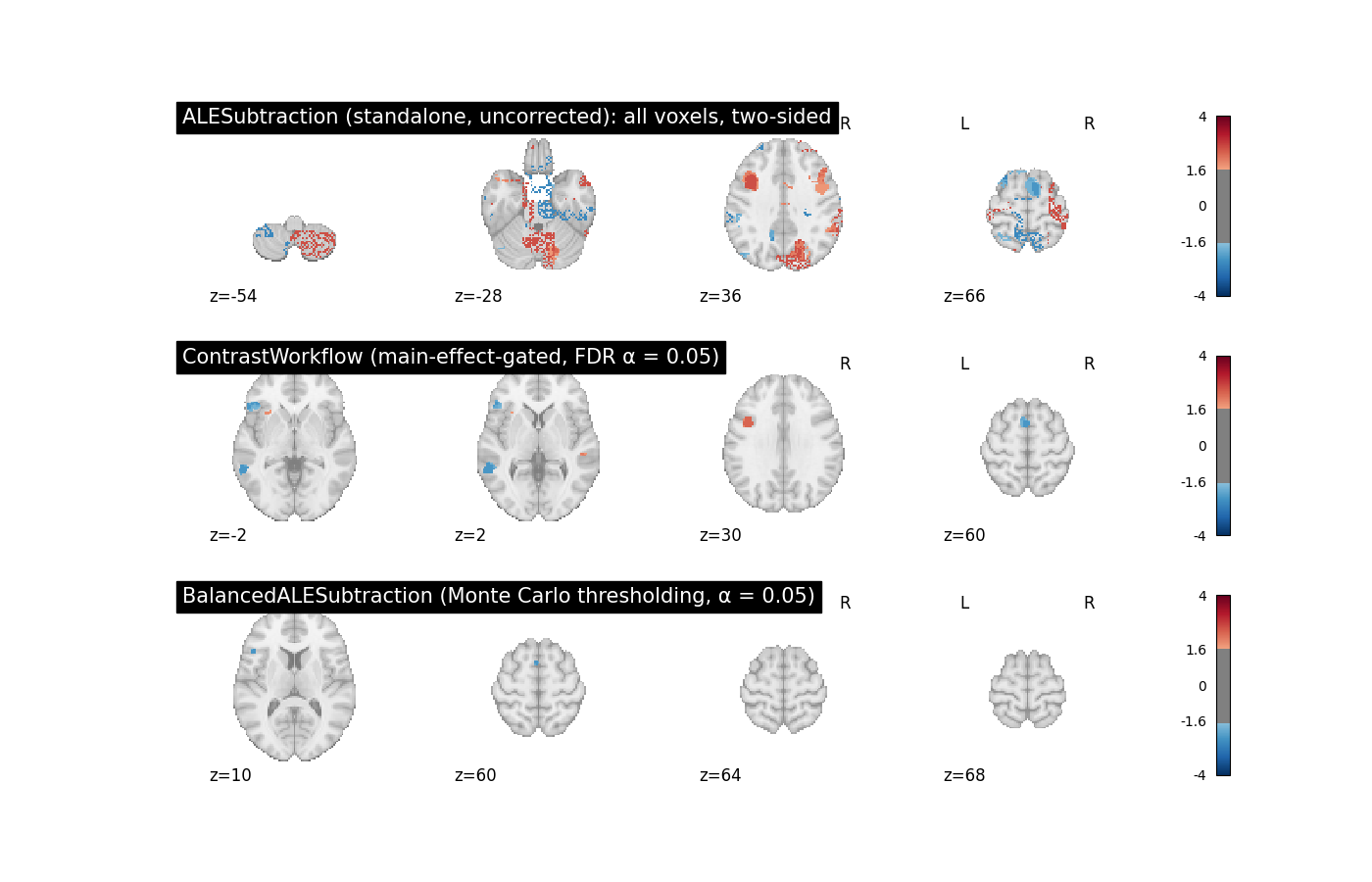
Side-by-side comparison of all three approaches

The three z-maps below show the same contrast (knowledge − relatedness) as estimated by each method. Differences in spatial extent and effect magnitude reflect whether directional masking or balanced sampling was applied.

fig4, axes4 = plt.subplots(figsize=(14, 9), nrows=3)

plot_stat_map(
    subtraction_result.get_map("z_desc-group1MinusGroup2"),
    cut_coords=4,
    display_mode="z",
    title="ALESubtraction (standalone, uncorrected): all voxels, two-sided",
    threshold=1.65,
    cmap="RdBu_r",
    symmetric_cbar=True,
    vmax=4,
    axes=axes4[0],
    figure=fig4,
)

plot_stat_map(
    contrast_result.get_map("z_desc-contrast"),
    cut_coords=4,
    display_mode="z",
    title="ContrastWorkflow (main-effect-gated, FDR α = 0.05)",
    threshold=1.65,
    cmap="RdBu_r",
    symmetric_cbar=True,
    vmax=4,
    axes=axes4[1],
    figure=fig4,
)

plot_stat_map(
    balanced_result.get_map("z_desc-balancedGroup1MinusGroup2"),
    cut_coords=4,
    display_mode="z",
    title="BalancedALESubtraction (Monte Carlo thresholding, α = 0.05)",
    threshold=1.65,
    cmap="RdBu_r",
    symmetric_cbar=True,
    vmax=4,
    axes=axes4[2],
    figure=fig4,
)

fig4.show()

Key differences at a glance

Feature	ALESubtraction	ContrastWorkflow	BalancedALESubtraction
Corrects for unequal group sizes	No	No	Yes (matched-size subsampling)
Computes group main effects	No	Yes (one-sample ALE per group)	Yes (probabilistic maps via subsampling)
Corrects main effects	No	Yes (FDR by default)	Yes (cluster threshold via Monte Carlo)
Directional inference masking	No — two-sided across all voxels	Yes — gated by thresholded main effects	No — prior-masked two-sided extrema null
Separate correction step needed	Yes (FWECorrector / FDRCorrector)	No additional corrector call (thresholding is internal)	No additional corrector call (Monte Carlo extrema thresholding)
Conjunction output	No	Yes (min of main-effect z-maps)	Yes (min of probability maps)
Output maps	z, p, logp for the difference	Main effects + conjunction z-maps + thresholded contrast	Balanced z/p/stat + probability maps + conjunction
Null model options	Label permutation (only)	Label permutation (only)	random-foci or label-permutation
Matches original GingerALE logic	No	GingerALE-style	No (new method)
Reference	—	Laird et al.[1]	Frahm et al.[2]

When to use each approach

• Use ALESubtraction (standalone) when you want a whole-mask, two-sided test without main-effect gating — for example during exploratory analyses or when you deliberately want to avoid pre-selecting regions based on each group’s main effect. It is the simplest option and requires applying a corrector to the result as a separate step. Avoid it when group sizes differ substantially, as the larger group will have systematically inflated ALE values.

• Use ContrastWorkflow when you want to mirror the original GingerALE-style subtraction logic and your group sizes are roughly equal. Restricting directional inference to regions where the respective group shows reliable activation reduces the risk of interpreting differences in regions that neither group activates consistently, and produces interpretable intermediate outputs (main effects, conjunction) alongside the final contrast. This is the closest NiMARE workflow for preregistered analyses that need GingerALE-style main-effect gating.

• Use BalancedALESubtraction when the two groups have unequal numbers of studies, or when you want a method that explicitly quantifies activation probability per group rather than just thresholded significance. The probabilistic activation maps and matched- size subsampling make this the most robust option for asymmetric literature searches. The internal Monte Carlo thresholding means no separate corrector call is needed, but computation time is substantially higher than the other two methods (controlled by n_subsamples, difference_iterations, and n_iters).

Boilerplate text and references

print("ContrastWorkflow description:")
pprint(contrast_result.description_)
print("\nBalancedALESubtraction description:")
pprint(balanced_result.description_)

ContrastWorkflow description:
('Group 1 main-effect analysis: An activation likelihood estimation (ALE) '
 'meta-analysis '
 '\\citep{turkeltaub2002meta,turkeltaub2012minimizing,eickhoff2012activation} '
 'was performed with NiMARE 0.20.0+2.gba8d921 (RRID:SCR_017398; '
 '\\citealt{Salo2023}), using a(n) ALE kernel. An ALE kernel '
 '\\citep{eickhoff2012activation} was used to generate study-wise modeled '
 'activation maps from coordinates. In this kernel method, each coordinate is '
 'convolved with a Gaussian kernel with full-width at half max values '
 'determined on a study-wise basis based on the study sample sizes according '
 'to the formulae provided in \\cite{eickhoff2012activation}. For voxels with '
 'overlapping kernels, the maximum value was retained. ALE values were '
 'converted to p-values using an approximate null distribution '
 '\\citep{eickhoff2012activation}. The input dataset included 262 foci from 21 '
 'experiments, with a total of 456 participants. False discovery rate '
 'correction was performed with the Benjamini-Hochberg procedure '
 '\\citep{benjamini1995controlling}. Group 2 main-effect analysis: An '
 'activation likelihood estimation (ALE) meta-analysis '
 '\\citep{turkeltaub2002meta,turkeltaub2012minimizing,eickhoff2012activation} '
 'was performed with NiMARE 0.20.0+2.gba8d921 (RRID:SCR_017398; '
 '\\citealt{Salo2023}), using a(n) ALE kernel. An ALE kernel '
 '\\citep{eickhoff2012activation} was used to generate study-wise modeled '
 'activation maps from coordinates. In this kernel method, each coordinate is '
 'convolved with a Gaussian kernel with full-width at half max values '
 'determined on a study-wise basis based on the study sample sizes according '
 'to the formulae provided in \\cite{eickhoff2012activation}. For voxels with '
 'overlapping kernels, the maximum value was retained. ALE values were '
 'converted to p-values using an approximate null distribution '
 '\\citep{eickhoff2012activation}. The input dataset included 201 foci from 16 '
 'experiments, with a total of 353 participants. False discovery rate '
 'correction was performed with the Benjamini-Hochberg procedure '
 '\\citep{benjamini1995controlling}. Pairwise contrast analysis: An activation '
 'likelihood estimation (ALE) subtraction analysis '
 '\\citep{laird2005ale,eickhoff2012activation} was performed with NiMARE '
 'v0.20.0+2.gba8d921 (RRID:SCR_017398; \\citealt{Salo2023}), using a(n) ALE '
 'kernel. An ALE kernel \\citep{eickhoff2012activation} was used to generate '
 'study-wise modeled activation maps from coordinates. In this kernel method, '
 'each coordinate is convolved with a Gaussian kernel with full-width at half '
 'max values determined on a study-wise basis based on the study sample sizes '
 'according to the formulae provided in \\cite{eickhoff2012activation}. For '
 'voxels with overlapping kernels, the maximum value was retained. The '
 "subtraction analysis was implemented according to NiMARE's \\citep{Salo2023} "
 'approach, which differs from the original version. In this version, '
 'ALE-difference scores are calculated between the two datasets, for all '
 'voxels in the mask, rather than for voxels significant in the main effects '
 'analyses of the two datasets. Next, voxel-wise null distributions of '
 'ALE-difference scores were generated via a randomized group assignment '
 'procedure, in which the studies in the two datasets were randomly reassigned '
 'and ALE-difference scores were calculated for the randomized datasets. This '
 'randomization procedure was repeated 100 times to build the null '
 'distributions. The significance of the original ALE-difference scores was '
 'assessed using a two-sided statistical test. The null distributions were '
 'assumed to be asymmetric, as ALE-difference scores will be skewed based on '
 'the sample sizes of the two datasets. The first input dataset (group1) '
 'included 262 foci from 21 experiments, with a total of 456 participants. The '
 'second input dataset (group2) included 201 foci from 16 experiments, with a '
 'total of 353 participants.  Masked contrast workflow: The group 1 and group '
 '2 main-effect maps were corrected with FDRCorrector and thresholded at alpha '
 '= 0.05. The thresholded main-effect maps were passed to ALESubtraction as '
 'directional inference masks. Positive group1 > group2 effects were evaluated '
 'only where group 1 had a surviving main effect, and negative group2 > group1 '
 'effects were evaluated only where group 2 had a surviving main effect. The '
 'pairwise contrast p-values were then thresholded at the same alpha level. '
 'The output includes the thresholded group main-effect maps, a '
 'voxelwise-minimum conjunction map, and the thresholded pairwise contrast '
 'map. This follows the main-effect-gated ALE subtraction logic used in '
 'earlier ALE subtraction workflows \\citep{laird2005ale} and the JALE '
 'implementation \\citep{Frahm_Monimu_Hoffstaedter}.')

BalancedALESubtraction description:
('A balanced ALE subtraction was performed in NiMARE using matched-size '
 'subsampling within groups, averaged balanced ALE differences, and Monte '
 'Carlo null extrema from balanced resamples. '
 ':footcite:t:`Frahm_Monimu_Hoffstaedter`')

References

[1] (1,2,3)

Angela R Laird, P Mickle Fox, Cathy J Price, David C Glahn, Angela M Uecker, Jack L Lancaster, Peter E Turkeltaub, Peter Kochunov, and Peter T Fox. Ale meta-analysis: controlling the false discovery rate and performing statistical contrasts. Human brain mapping, 25(1):155–164, 2005. URL: https://doi.org/10.1002/hbm.20136, doi:10.1002/hbm.20136.

[2] (1,2,3,4)

Lennart Frahm, Monimu, and Felix Hoffstaedter. Juaml/jale. URL: https://github.com/juaml/JALE.

[3]

Alexander Enge, Rasha Abdel Rahman, and Michael A Skeide. A meta-analysis of fmri studies of semantic cognition in children. NeuroImage, 241:118436, 2021. URL: https://doi.org/10.1016/j.neuroimage.2021.118436, doi:10.1016/j.neuroimage.2021.118436.