The Cognitive Atlas

Download the Cognitive Atlas and extract CogAt terms from text.

import os

import matplotlib.pyplot as plt
import numpy as np
import pandas as pd

from nimare import annotate, extract
from nimare.nimads import Studyset
from nimare.utils import get_resource_path

Load Studyset with abstracts

studyset = Studyset(
    os.path.join(get_resource_path(), "neurosynth_laird_studyset.json"),
    target="mni152_2mm",
)

Download Cognitive Atlas

cogatlas = extract.download_cognitive_atlas(data_dir=get_resource_path(), overwrite=False)
id_df = pd.read_csv(cogatlas["ids"])
rel_df = pd.read_csv(cogatlas["relationships"])

ID DataFrame

id_df.head()

	id	name	alias	length	ratio
0	tsk_4a57abb949e35	structured clinical interview for diagnostic a...	structured clinical interview for diagnostic a...	96.0	100
1	tsk_4a57abb949e35	structured clinical interview for diagnostic a...	dsm-iv structured clinical interview for diagn...	94.0	92
2	tsk_4a57abb949e35	structured clinical interview for diagnostic a...	structured clinical interview for diagnostic a...	87.0	95
3	trm_5176cf9d3d512	living/nonliving judgment on mirror-reversed a...	living/nonliving judgment on mirror-reversed a...	65.0	100
4	trm_56a2b7c08a279	short penn continuous performance test-number ...	short penn continuous performance test-number ...	64.0	100

Relationships DataFrame

rel_df.head()

	input	output	rel_type
0	trm_4a3fd79d096be	ctp_C3	inCategory
1	trm_4a3fd79d096e3	ctp_C3	inCategory
2	trm_4a3fd79d096f0	ctp_C3	inCategory
3	trm_4a3fd79d096fc	ctp_C1	inCategory
4	trm_4a3fd79d09707	ctp_C1	inCategory

Extract Cognitive Atlas terms from text

counts_df, rep_text_df = annotate.cogat.extract_cogat(
    studyset.texts,
    id_df,
    text_column="abstract",
)

Expand counts

weights = {"isKindOf": 1, "isPartOf": 1, "inCategory": 1}
expanded_df = annotate.cogat.expand_counts(counts_df, rel_df, weights)
# Sort by total count and reduce for better visualization
series = expanded_df.sum(axis=0)
series = series.sort_values(ascending=False)
series = series[series > 0]
columns = series.index.tolist()

Add annotations to the Studyset

Now we can add the generated annotations back into the Studyset object. We’ll use the expanded counts since they provide more comprehensive annotations. The annotation functions return DataFrames with ‘id’ as the index, so we need to reset the index to make ‘id’ a column before assigning to the Studyset.

This will replace any existing annotations. If you want to add to existing annotations instead of replacing them, you can merge the DataFrames: studyset.annotations_df = studyset.annotations_df.merge(expanded_df.reset_index(), on='id', how='left')

studyset.annotations_df = expanded_df.reset_index()

# Now the Studyset has the new annotations
print(f"Studyset now has {len(studyset.annotations_df.columns)} annotation columns")

Studyset now has 1792 annotation columns

Make some plots

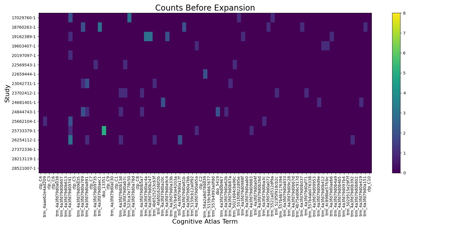
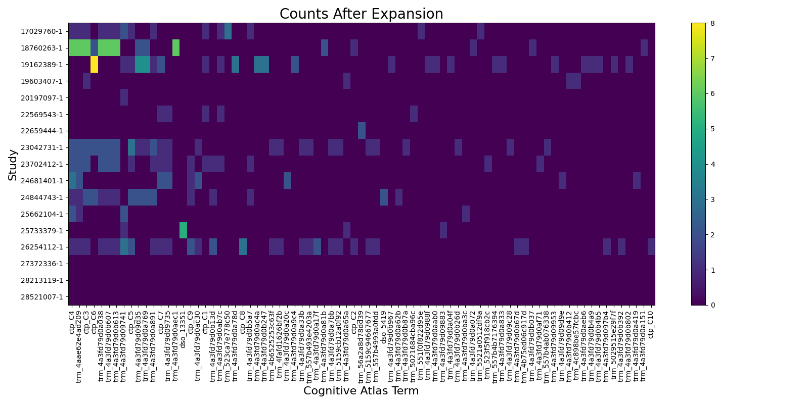
We will reduce the dataframes to only columns with at least one count to make visualization easier.

# Raw counts
fig1, ax1 = plt.subplots(figsize=(16, 8))
pos = ax1.imshow(counts_df[columns].values, aspect="auto", vmin=0, vmax=np.max(expanded_df.values))
fig1.colorbar(pos, ax=ax1)
ax1.set_title("Counts Before Expansion", fontsize=20)
ax1.set_yticks(range(counts_df.shape[0]))
ax1.set_yticklabels(counts_df.index)
ax1.set_ylabel("Study", fontsize=16)
ax1.set_xticks(range(len(columns)))
ax1.set_xticklabels(columns, rotation=90)
ax1.set_xlabel("Cognitive Atlas Term", fontsize=16)
fig1.tight_layout()
fig1.show()

# Expanded counts
fig2, ax2 = plt.subplots(figsize=(16, 8))
pos = ax2.imshow(
    expanded_df[columns].values, aspect="auto", vmin=0, vmax=np.max(expanded_df.values)
)
fig2.colorbar(pos, ax=ax2)
ax2.set_title("Counts After Expansion", fontsize=20)
ax2.set_yticks(range(counts_df.shape[0]))
ax2.set_yticklabels(counts_df.index)
ax2.set_ylabel("Study", fontsize=16)
ax2.set_xticks(range(len(columns)))
ax2.set_xticklabels(columns, rotation=90)
ax2.set_xlabel("Cognitive Atlas Term", fontsize=16)
fig2.tight_layout()
fig2.show()

• 
•