GCLDA topic modeling

Train a generalized correspondence latent Dirichlet allocation model using abstracts.

Warning

The model in this example is trained using (1) a very small, nonrepresentative dataset and (2) very few iterations. As such, it will not provide useful results. If you are interested in using GCLDA, we recommend using a large dataset like Neurosynth, and training with at least 10k iterations.

import os

import nibabel as nib
import numpy as np
from nilearn import image, masking, plotting

from nimare import annotate, decode
from nimare.dataset import Dataset
from nimare.utils import get_resource_path

Load dataset with abstracts

We’ll load a small dataset composed only of studies in Neurosynth with Angela Laird as a coauthor, for the sake of speed.

dset = Dataset(os.path.join(get_resource_path(), "neurosynth_laird_studies.json"))
dset.texts.head(2)

	id	study_id	contrast_id	abstract
0	17029760-1	17029760	1	Repetitive transcranial magnetic stimulation (...
1	18760263-1	18760263	1	In an effort to clarify how deductive reasonin...

Generate term counts

GCLDA uses raw word counts instead of the tf-idf values generated by Neurosynth.

counts_df = annotate.text.generate_counts(
    dset.texts,
    text_column="abstract",
    tfidf=False,
    max_df=0.99,
    min_df=0.01,
)
counts_df.head(5)

	10	10 brains	10 located	11	11 published	11 showing	17	17 sca17	2005	2005 major	2012	2012 evidence	aberrant	aberrant hotspots	abilities	abilities action	abnormal	abnormal sexual	abnormal structure	abstract	abstract cognitive	abstract emulation	accessible	accessible ensuing	accompanied	accompanied differential	accomplished	accomplished substrates	account	account common	accurate	accurate robust	acetylcholine	acetylcholine receptor	acquired	acquired standard	action	action cognition	action selection	activating	...	versus	versus baseline	vi	vi extent	vi ix	viewed	viewed problem	viib	viib viiia	viiia	viiia viiib	viiib	viiib cerebellar	vmpfc	vmpfc pcc	vmpfc posterior	vocalization	vocalization altered	voice	voice control	voice network	voice perturbation	vowel	vowel phonation	voxel	voxel applying	voxel morphometry	voxel syllable	voxels	voxels fp	way	way disrupted	weaknesses	weaknesses conventional	wernicke	wernicke responded	widespread	widespread functional	working	working memory
id
17029760-1	0	0	0	0	0	0	0	0	1	1	0	0	0	0	0	0	0	0	0	0	0	0	0	0	0	0	0	0	0	0	0	0	0	0	0	0	0	0	0	0	...	0	0	0	0	0	0	0	0	0	0	0	0	0	0	0	0	0	0	0	0	0	0	0	0	0	0	0	0	0	0	0	0	0	0	0	0	0	0	0	0
18760263-1	0	0	0	0	0	0	0	0	0	0	0	0	0	0	0	0	0	0	0	0	0	0	0	0	0	0	1	1	0	0	0	0	0	0	0	0	0	0	0	0	...	0	0	0	0	0	1	1	0	0	0	0	0	0	0	0	0	0	0	0	0	0	0	0	0	0	0	0	0	0	0	0	0	0	0	1	1	0	0	0	0
19162389-1	0	0	0	2	1	1	0	0	0	0	0	0	0	0	0	0	0	0	0	0	0	0	0	0	0	0	0	0	0	0	0	0	0	0	0	0	0	0	0	0	...	0	0	0	0	0	0	0	0	0	0	0	0	0	0	0	0	0	0	0	0	0	0	1	1	1	0	0	1	0	0	0	0	0	0	0	0	0	0	0	0
19603407-1	0	0	0	0	0	0	0	0	0	0	0	0	0	0	0	0	0	0	0	0	0	0	0	0	0	0	0	0	0	0	1	1	0	0	0	0	0	0	0	0	...	0	0	0	0	0	0	0	0	0	0	0	0	0	0	0	0	0	0	0	0	0	0	0	0	0	0	0	0	0	0	0	0	1	1	0	0	0	0	0	0
20197097-1	0	0	0	0	0	0	0	0	0	0	0	0	0	0	0	0	0	0	0	0	0	0	0	0	0	0	0	0	0	0	0	0	0	0	1	1	0	0	0	0	...	0	0	0	0	0	0	0	0	0	0	0	0	0	0	0	0	0	0	0	0	0	0	0	0	0	0	0	0	0	0	0	0	0	0	0	0	0	0	0	0

5 rows × 2520 columns

Run model

Five iterations will take ~10 minutes with the full Neurosynth dataset. It’s much faster with this reduced example dataset. Note that we’re using only 10 topics here. This is because there are only 13 studies in the dataset. If the number of topics is higher than the number of studies in the dataset, errors can occur during training.

model = annotate.gclda.GCLDAModel(
    counts_df,
    dset.coordinates,
    mask=dset.masker.mask_img,
    n_topics=10,
    n_regions=4,
    symmetric=True,
)
model.fit(n_iters=100, loglikely_freq=20)
model.save("gclda_model.pkl.gz")

# Let's remove the model now that you know how to generate it.
os.remove("gclda_model.pkl.gz")

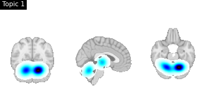
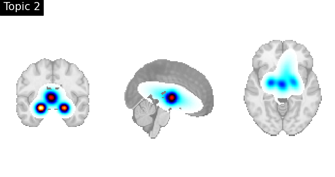
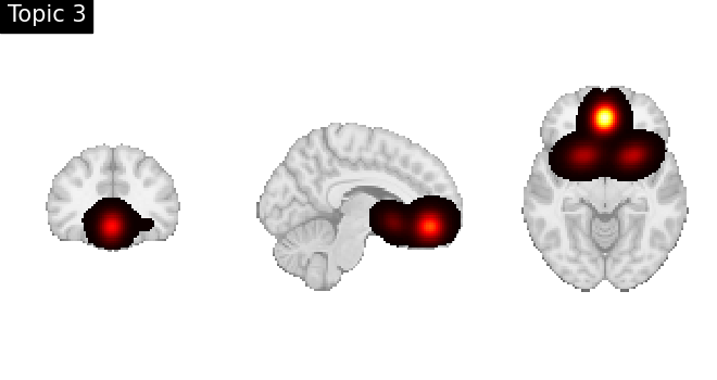
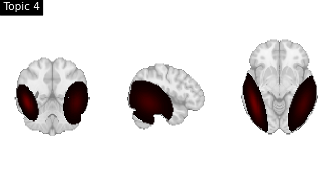
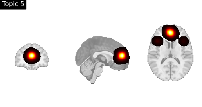
Look at topics

topic_img_4d = masking.unmask(model.p_voxel_g_topic_.T, model.mask)
for i_topic in range(5):
    topic_img_3d = image.index_img(topic_img_4d, i_topic)
    plotting.plot_stat_map(
        topic_img_3d,
        draw_cross=False,
        colorbar=False,
        annotate=False,
        title=f"Topic {i_topic + 1}",
    )

• 
• 
• 
• 
• 

Generate a pseudo-statistic image from text

text = "dorsal anterior cingulate cortex"
encoded_img, _ = decode.encode.gclda_encode(model, text)
plotting.plot_stat_map(encoded_img, draw_cross=False)

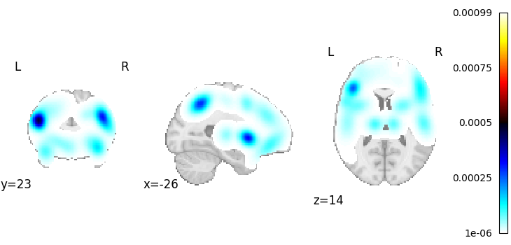
<nilearn.plotting.displays._slicers.OrthoSlicer object at 0x7fe923f14f70>

Decode an unthresholded statistical map

For the sake of simplicity, we will use the pseudo-statistic map generated in the previous step.

# Run the decoder
decoded_df, _ = decode.continuous.gclda_decode_map(model, encoded_img)
decoded_df.sort_values(by="Weight", ascending=False).head(10)

	Weight
Term
functions	0.053079
cognition	0.053079
pmd	0.047181
cortex	0.042285
networks	0.037038
anterior	0.035490
fp	0.030304
frontal	0.029671
cbp	0.029488
functionally	0.029488

Decode an ROI image

First we’ll make an ROI

arr = np.zeros(dset.masker.mask_img.shape, np.int32)
arr[65:75, 50:60, 50:60] = 1
mask_img = nib.Nifti1Image(arr, dset.masker.mask_img.affine)
plotting.plot_roi(mask_img, draw_cross=False)

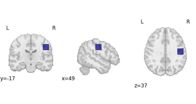
<nilearn.plotting.displays._slicers.OrthoSlicer object at 0x7fe923b7b850>

Run the decoder

decoded_df, _ = decode.discrete.gclda_decode_roi(model, mask_img)
decoded_df.sort_values(by="Weight", ascending=False).head(10)

	Weight
Term
motor	24.666614
seed	20.181775
structural	17.939355
cortex	15.722663
behavioral	15.696936
methods	11.237680
speech	11.218747
connectivity modeling	11.212097
sca17	11.212097
connectivity patterns	8.969678