Coordinate-based meta-regression algorithms

A tour of Coordinate-based meta-regression (CBMR) algorithms in NiMARE.

CBMR is a generative framework to approximate smooth activation intensity function and investigate the effect of study-level moderators (e.g., year of pubilication, sample size, subtype of stimuli). CBMR considers three stochastic models (Poisson, Negative Binomial (NB) and Clustered NB) for modeling the random variation in foci, and allows flexible statistical inference for either spatial homogeneity tests or group comparison tests. It is a computationally efficient approach with good statistical interpretability to model the locations of activation foci.

This tutorial is intended to provide a brief description and example of the CBMR algorithm implemented in NiMARE.

For a more detailed introduction to the elements of a coordinate-based meta-regression, see the online course or a brief overview.

import numpy as np
import scipy
from nilearn.plotting import plot_stat_map

from nimare.generate import create_coordinate_studyset
from nimare.meta import models
from nimare.transforms import StandardizeField

Load Studyset-compatible data

Here, we’re going to simulate a dataset (using nimare.generate.create_coordinate_dataset that includes 100 studies, each with 10 reported foci and sample size varying between 20 and 40. We separate them into four groups according to diagnosis (schizophrenia or depression) and drug status (Yes or No). We also add two continuous study-level moderators (sample size and average age) and a categorical study-level moderator (schizophrenia subtype).

# data simulation
ground_truth_foci, studyset = create_coordinate_studyset(
    foci=10,
    sample_size=(20, 40),
    n_studies=1000,
)
# set up group columns: diagnosis & drug_status
annotations_df = studyset.annotations_df.copy()
n_rows = annotations_df.shape[0]
annotations_df["diagnosis"] = [
    "schizophrenia" if i % 2 == 0 else "depression" for i in range(n_rows)
]
annotations_df["drug_status"] = ["Yes" if i % 2 == 0 else "No" for i in range(n_rows)]
annotations_df["drug_status"] = (
    annotations_df["drug_status"].sample(frac=1).reset_index(drop=True)
)  # random shuffle drug_status column
# set up continuous moderators: sample sizes & avg_age
annotations_df["sample_sizes"] = [studyset.metadata.sample_sizes[i][0] for i in range(n_rows)]
annotations_df["avg_age"] = np.arange(n_rows)
# set up categorical moderators: schizophrenia_subtype (as not enough data to be interpreted
# as groups)
annotations_df["schizophrenia_subtype"] = ["type1", "type2", "type3", "type4", "type5"] * int(
    n_rows / 5
)
annotations_df["schizophrenia_subtype"] = (
    annotations_df["schizophrenia_subtype"].sample(frac=1).reset_index(drop=True)
)  # random shuffle drug_status column
studyset.annotations_df = annotations_df

Estimation of group-specific spatial intensity functions

CBMR can generate estimates of group-specific spatial intensity functions for multiple groups simultaneously, with different group-specific spatial regression coefficients.

CBMR can also consider the effects of study-level moderators (e.g. sample size, year of publication) by estimating regression coefficients of moderators (shared by all groups).

Note that study-level moderators can only have global effects instead of localized effects within CBMR framework. In the scenario that there are multiple subgroups within a group (e.g., indexed as subgroup-1 to subgroup-n, but one or more of them don’t have enough number of studies to be inferred as a separate group). Using categorical encoding, CBMR can interpret the subgroups as categorical moderators for each study (either 0 or 1), and estimate the global activation intensity associated with each subgroup (comparing to the average).

from nimare.meta import CBMREstimator

studyset = StandardizeField(fields=["sample_sizes", "avg_age"]).transform(studyset)

cbmr = CBMREstimator(
    group_categories=["diagnosis", "drug_status"],
    moderators=[
        "standardized_sample_sizes",
        "standardized_avg_age",
        "schizophrenia_subtype:reference=type1",
    ],
    spline_spacing=100,  # a reasonable choice is 10 or 5, 100 is for speed
    model=models.PoissonEstimator,
    penalty=False,
    lr=1e-1,
    tol=1e3,  # a reasonable choice is 1e-2, 1e3 is for speed
    device="cpu",  # "cuda" if you have GPU
)
results = cbmr.fit(dataset=studyset)

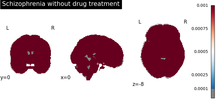
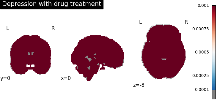
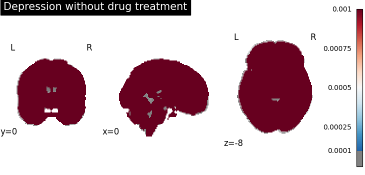
Now that we have fitted the model, we can plot the spatial intensity maps.

plot_stat_map(
    results.get_map("spatialIntensity_group-SchizophreniaYes"),
    cut_coords=[0, 0, -8],
    draw_cross=False,
    cmap="RdBu_r",
    symmetric_cbar=True,
    title="Schizophrenia with drug treatment",
    threshold=1e-4,
    vmax=1e-3,
)
plot_stat_map(
    results.get_map("spatialIntensity_group-SchizophreniaNo"),
    cut_coords=[0, 0, -8],
    draw_cross=False,
    cmap="RdBu_r",
    symmetric_cbar=True,
    title="Schizophrenia without drug treatment",
    threshold=1e-4,
    vmax=1e-3,
)
plot_stat_map(
    results.get_map("spatialIntensity_group-DepressionYes"),
    cut_coords=[0, 0, -8],
    draw_cross=False,
    cmap="RdBu_r",
    symmetric_cbar=True,
    title="Depression with drug treatment",
    threshold=1e-4,
    vmax=1e-3,
)
plot_stat_map(
    results.get_map("spatialIntensity_group-DepressionNo"),
    cut_coords=[0, 0, -8],
    draw_cross=False,
    cmap="RdBu_r",
    symmetric_cbar=True,
    title="Depression without drug treatment",
    threshold=1e-4,
    vmax=1e-3,
)

• 
• 
• 
• 

<nilearn.plotting.displays._slicers.OrthoSlicer object at 0x784a7ea5fc20>

Four figures correspond to group-specific spatial intensity map of four groups (“schizophreniaYes”, “schizophreniaNo”, “depressionYes”, “depressionNo”). Areas with stronger spatial intensity are highlighted.

Generalized Linear Hypothesis (GLH) testing for spatial homogeneity

In the most basic scenario of spatial homogeneity testing, the fitted CBMR result can run inference directly. The available groups and moderators are discoverable from the result.

print(results.describe_inference_inputs())
contrast_result = results.test_groups()

{'groups': ('SchizophreniaYes', 'DepressionYes', 'SchizophreniaNo', 'DepressionNo'), 'moderators': ('standardized_sample_sizes', 'standardized_avg_age', 'type2', 'type3', 'type4', 'type5')}

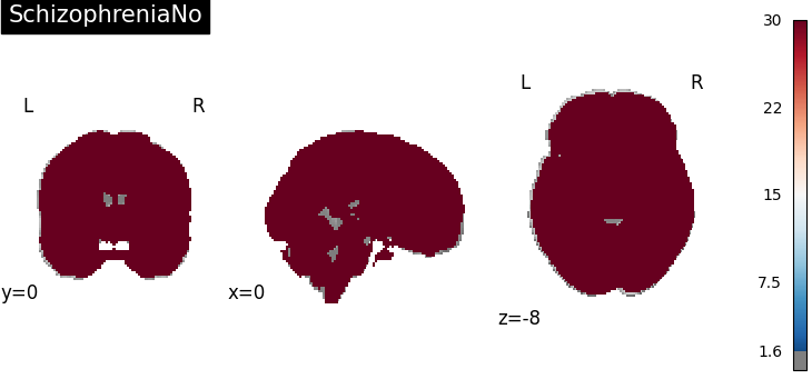
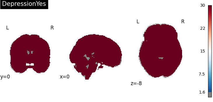
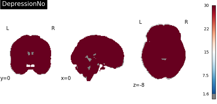
Now that we have done spatial homogeneity tests, we can plot the z-score maps.

# generate z-score maps for group-wise spatial homogeneity test
plot_stat_map(
    contrast_result.get_map("z_group-SchizophreniaYes"),
    cut_coords=[0, 0, -8],
    draw_cross=False,
    cmap="RdBu_r",
    symmetric_cbar=True,
    title="SchizophreniaYes",
    threshold=scipy.stats.norm.isf(0.05),
    vmax=30,
)

plot_stat_map(
    contrast_result.get_map("z_group-SchizophreniaNo"),
    cut_coords=[0, 0, -8],
    draw_cross=False,
    cmap="RdBu_r",
    symmetric_cbar=True,
    title="SchizophreniaNo",
    threshold=scipy.stats.norm.isf(0.05),
    vmax=30,
)

plot_stat_map(
    contrast_result.get_map("z_group-DepressionYes"),
    cut_coords=[0, 0, -8],
    draw_cross=False,
    cmap="RdBu_r",
    symmetric_cbar=True,
    title="DepressionYes",
    threshold=scipy.stats.norm.isf(0.05),
    vmax=30,
)

plot_stat_map(
    contrast_result.get_map("z_group-DepressionNo"),
    cut_coords=[0, 0, -8],
    draw_cross=False,
    cmap="RdBu_r",
    symmetric_cbar=True,
    title="DepressionNo",
    threshold=scipy.stats.norm.isf(0.05),
    vmax=30,
)

• 
• 
• 
• 

<nilearn.plotting.displays._slicers.OrthoSlicer object at 0x784a7acd1390>

Four figures (displayed as z-statistics map) correspond to homogeneity test of group-specific spatial intensity for four groups. The null hypothesis assumes homogeneous spatial intensity over the whole brain, , , where is the number of voxels within brain mask, is the index of voxel. Areas with significant p-values are highlighted (under significance level ).

Perform false discovery rate (FDR) correction on spatial homogeneity test

The default FDR correction method is “indep”, using Benjamini-Hochberg(BH) procedure.

from nimare.correct import FDRCorrector

corr = FDRCorrector(method="indep", alpha=0.05)
cres = corr.transform(contrast_result)

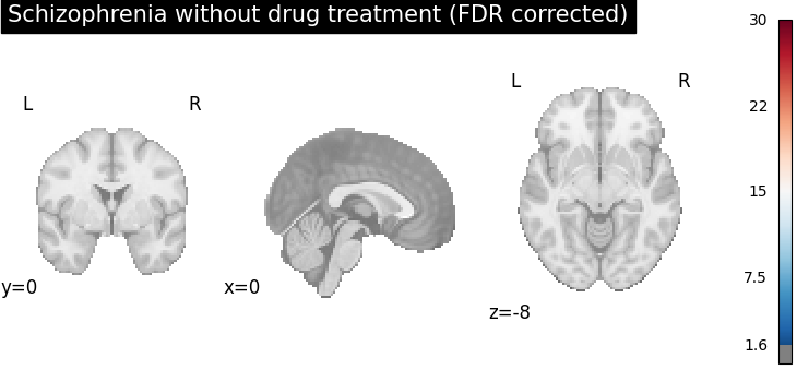
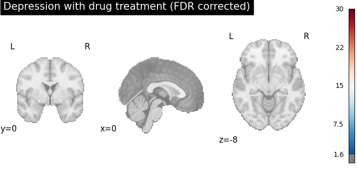
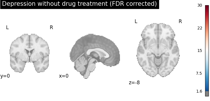
Now that we have applied the FDR correction methods, we can plot the FDR corrected z-score maps.

# generate FDR corrected z-score maps for group-wise spatial homogeneity test
plot_stat_map(
    cres.get_map("z_group-SchizophreniaYes_corr-FDR_method-indep"),
    cut_coords=[0, 0, -8],
    draw_cross=False,
    cmap="RdBu_r",
    symmetric_cbar=True,
    title="Schizophrenia with drug treatment (FDR corrected)",
    threshold=scipy.stats.norm.isf(0.05),
    vmax=30,
)

plot_stat_map(
    cres.get_map("z_group-SchizophreniaNo_corr-FDR_method-indep"),
    cut_coords=[0, 0, -8],
    draw_cross=False,
    cmap="RdBu_r",
    symmetric_cbar=True,
    title="Schizophrenia without drug treatment (FDR corrected)",
    threshold=scipy.stats.norm.isf(0.05),
    vmax=30,
)

plot_stat_map(
    cres.get_map("z_group-DepressionYes_corr-FDR_method-indep"),
    cut_coords=[0, 0, -8],
    draw_cross=False,
    cmap="RdBu_r",
    symmetric_cbar=True,
    title="Depression with drug treatment (FDR corrected)",
    threshold=scipy.stats.norm.isf(0.05),
    vmax=30,
)

plot_stat_map(
    cres.get_map("z_group-DepressionNo_corr-FDR_method-indep"),
    cut_coords=[0, 0, -8],
    draw_cross=False,
    cmap="RdBu_r",
    symmetric_cbar=True,
    title="Depression without drug treatment (FDR corrected)",
    threshold=scipy.stats.norm.isf(0.05),
    vmax=30,
)

• 
• 
• 
• 

<nilearn.plotting.displays._slicers.OrthoSlicer object at 0x784a7acd31d0>

After FDR correction (via BH procedure), areas with stronger spatial intensity are more stringent, (the number of voxels with significant p-values is reduced).

GLH testing for group comparisons among any two groups

Pairwise group comparisons can also be expressed more directly with tuples.

contrast_result = results.compare_groups(
    [
        ("SchizophreniaYes", "SchizophreniaNo"),
        ("SchizophreniaNo", "DepressionNo"),
        ("DepressionYes", "DepressionNo"),
    ]
)

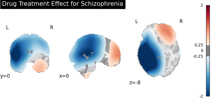
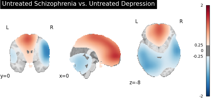
Now that we have done group comparison tests, we can plot the z-score maps indicating difference in spatial intensity between two groups.

# generate z-statistics maps for each group
plot_stat_map(
    contrast_result.get_map("z_group-SchizophreniaYes-SchizophreniaNo"),
    cut_coords=[0, 0, -8],
    draw_cross=False,
    cmap="RdBu_r",
    symmetric_cbar=True,
    title="Drug Treatment Effect for Schizophrenia",
    threshold=scipy.stats.norm.isf(0.4),
    vmax=2,
)

plot_stat_map(
    contrast_result.get_map("z_group-SchizophreniaNo-DepressionNo"),
    cut_coords=[0, 0, -8],
    draw_cross=False,
    cmap="RdBu_r",
    symmetric_cbar=True,
    title="Untreated Schizophrenia vs. Untreated Depression",
    threshold=scipy.stats.norm.isf(0.4),
    vmax=2,
)

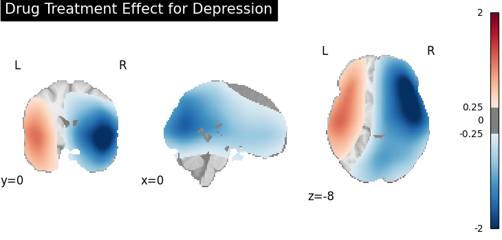
plot_stat_map(
    contrast_result.get_map("z_group-DepressionYes-DepressionNo"),
    cut_coords=[0, 0, -8],
    draw_cross=False,
    cmap="RdBu_r",
    symmetric_cbar=True,
    title="Drug Treatment Effect for Depression",
    threshold=scipy.stats.norm.isf(0.4),
    vmax=2,
)

• 
• 
• 

<nilearn.plotting.displays._slicers.OrthoSlicer object at 0x784a7a308940>

Four figures (displayed as z-statistics map) correspond to group comparison test of spatial intensity for any two groups. The null hypothesis assumes spatial intensity estimations of two groups are equal at voxel level, , , where is number of voxels within brain mask, is the index of voxel. Areas with significant p-values (significant difference in spatial intensity estimation between two groups) are highlighted (under significance level ).

GLH testing with contrast matrix specified

CBMR supports more flexible GLH tests by specifying contrast vectors or matrices directly through the result-level infer API. For example, the group comparison 2xgroup_0-1xgroup_1-1xgroup_2 can be represented as group_contrasts=[[2, -1, -1, 0]]. Multiple independent GLH tests can be conducted simultaneously by including multiple contrast vectors or matrices in group_contrasts.

CBMR also allows simultaneous GLH tests consisting of multiple contrast vectors, represented as one element of group_contrasts. Only if all of null hypotheses are rejected at voxel level, p-values are significant. For example, [[1, -1, 0, 0], [1, 0, -1, 0], [0, 0, 1, -1]] tests the equality of spatial intensity estimates across all four groups (finding consistent activation regions). Note that only contrast vectors are necessary for testing the equality of groups.

contrast_result = results.infer(
    group_contrasts=[[[1, -1, 0, 0], [1, 0, -1, 0], [0, 0, 1, -1]]],
    moderator_contrasts=False,
)

Now that we have done group comparison tests with the specified contrast matrix, we can plot the z-score maps indicating uniformity in activation regions among all four groups.

plot_stat_map(
    contrast_result.get_map("z_GLH_groups_0"),
    cut_coords=[0, 0, -8],
    draw_cross=False,
    cmap="RdBu_r",
    symmetric_cbar=True,
    title="GLH_groups_0",
    threshold=scipy.stats.norm.isf(0.4),
)
print("The contrast matrix of GLH_0 is {}".format(contrast_result.metadata["GLH_groups_0"]))

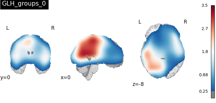
The contrast matrix of GLH_0 is [[ 1 -1  0  0]
 [ 1  0 -1  0]
 [ 0  0  1 -1]]

GLH testing for study-level moderators

The CBMR framework can estimate global study-level moderator effects and allows inference on whether those moderator effects differ from zero.

contrast_result = results.test_moderators()
print(contrast_result.tables["moderators_regression_coef"])
print(
    "P-values of moderator effects `sample_sizes` is {}".format(
        contrast_result.tables["p_standardized_sample_sizes"]
    )
)
print(
    "P-value of moderator effects `avg_age` is {}".format(
        contrast_result.tables["p_standardized_avg_age"]
    )
)

   standardized_sample_sizes  standardized_avg_age  ...    type4     type5
0                   0.004552              0.007163  ... -0.44846 -0.451156

[1 rows x 6 columns]
P-values of moderator effects `sample_sizes` is                p
0  4.940656e-324
P-value of moderator effects `avg_age` is                p
0  4.940656e-324

This table shows the regression coefficients of study-level moderators, here, sample_sizes and avg_age are standardized in the preprocessing steps. Moderator effects of both sample_size and avg_age are not significant under significance level . With reference to spatial intensity estimation of a chosen subtype, spatial intensity estimations of the other subtypes of schizophrenia are moderatored globally.

contrast_result = results.compare_moderators(
    [("standardized_sample_sizes", "standardized_avg_age")]
)
print(
    "P-values of the difference between two moderator effects (`sample_size-avg_age`) is {}".format(
        contrast_result.tables["p_standardized_sample_sizes-standardized_avg_age"]
    )
)

P-values of the difference between two moderator effects (`sample_size-avg_age`) is                p
0  4.727612e-121

CBMR also allows flexible contrasts between study-level covariates. For example, we can express the comparison standardized_sample_sizes-standardized_avg_age directly through results.compare_moderators(…) when exploring whether the moderator effects of sample_sizes and avg_age are equivalent.