Note
Go to the end to download the full example code.
Run a coordinate-based meta-analysis (CBMA) workflow
NiMARE provides a plethora of tools for performing meta-analyses on neuroimaging data. Sometimes it’s difficult to know where to start, especially if you’re new to meta-analysis. This tutorial will walk you through using a CBMA workflow function which puts together the fundamental steps of a CBMA meta-analysis.
import os
from pathlib import Path

import matplotlib.pyplot as plt
from nilearn.plotting import plot_stat_map

from nimare.nimads import Studyset
from nimare.reports.base import run_reports
from nimare.utils import get_resource_path
from nimare.workflows.cbma import CBMAWorkflow
Load Studyset
studyset_file = os.path.join(get_resource_path(), "nidm_pain_studyset.json")
studyset = Studyset(studyset_file, target="mni152_2mm")
Run CBMA Workflow
The fit method of a CBMA workflow class runs the following steps:
Runs a meta-analysis using the specified method (default: ALE)
Applies a corrector to the meta-analysis results (default: FWECorrector, montecarlo)
Generates cluster tables and runs diagnostics on the corrected results (default: Jackknife)
All in one call!
result = CBMAWorkflow().fit(studyset)
For this example, we use an FDR correction because the default corrector (FWE correction with Monte Carlo simulation) takes a long time to run due to the high number of iterations that are required
workflow = CBMAWorkflow(corrector="fdr")
result = workflow.fit(studyset)
  0%|          | 0/21 [00:00<?, ?it/s]
  5%|▍         | 1/21 [00:00<00:05,  3.72it/s]
 10%|▉         | 2/21 [00:00<00:05,  3.71it/s]
 14%|█▍        | 3/21 [00:00<00:04,  3.70it/s]
 19%|█▉        | 4/21 [00:01<00:04,  3.69it/s]
 24%|██▍       | 5/21 [00:01<00:04,  3.70it/s]
 29%|██▊       | 6/21 [00:01<00:04,  3.70it/s]
 33%|███▎      | 7/21 [00:01<00:03,  3.69it/s]
 38%|███▊      | 8/21 [00:02<00:03,  3.69it/s]
 43%|████▎     | 9/21 [00:02<00:03,  3.69it/s]
 48%|████▊     | 10/21 [00:02<00:02,  3.69it/s]
 52%|█████▏    | 11/21 [00:02<00:02,  3.66it/s]
 57%|█████▋    | 12/21 [00:03<00:02,  3.68it/s]
 62%|██████▏   | 13/21 [00:03<00:02,  3.68it/s]
 67%|██████▋   | 14/21 [00:03<00:01,  3.68it/s]
 71%|███████▏  | 15/21 [00:04<00:01,  3.68it/s]
 76%|███████▌  | 16/21 [00:04<00:01,  3.66it/s]
 81%|████████  | 17/21 [00:04<00:01,  3.67it/s]
 86%|████████▌ | 18/21 [00:04<00:00,  3.66it/s]
 90%|█████████ | 19/21 [00:05<00:00,  3.66it/s]
 95%|█████████▌| 20/21 [00:05<00:00,  3.68it/s]
100%|██████████| 21/21 [00:05<00:00,  3.69it/s]
100%|██████████| 21/21 [00:05<00:00,  3.68it/s]
Plot Results
The fit method of the CBMA workflow class returns a MetaResult object,
where you can access the corrected results of the meta-analysis and diagnostics tables.
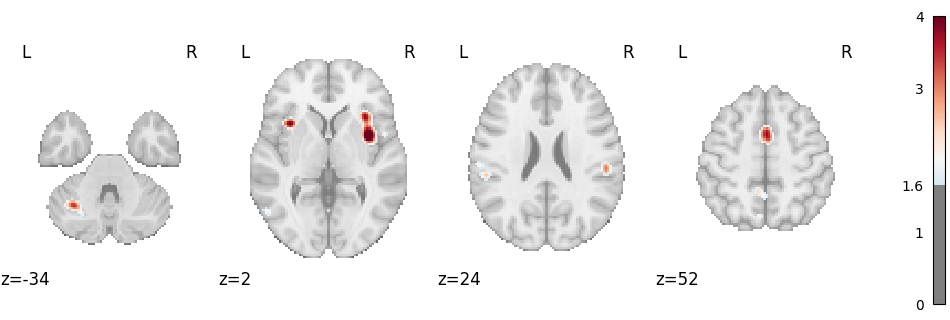
Corrected map:
img = result.get_map("z_corr-FDR_method-indep")
plot_stat_map(
    img,
    cut_coords=4,
    display_mode="z",
    threshold=1.65,  # voxel_thresh p < .05, one-tailed
    cmap="RdBu_r",
    symmetric_cbar=True,
    vmax=4,
)
plt.show()
Clusters table
result.tables["z_corr-FDR_method-indep_tab-clust"]
Contribution table
result.tables["z_corr-FDR_method-indep_diag-Jackknife_tab-counts_tail-positive"]
Report
Finally, a NiMARE report is generated from the MetaResult. root_dir = Path(os.getcwd()).parents[1] / “docs” / “_build” Use the previous root to run the documentation locally.
root_dir = Path(os.getcwd()).parents[1] / "_readthedocs"
html_dir = root_dir / "html" / "auto_examples" / "02_meta-analyses" / "10_plot_cbma_workflow"
html_dir.mkdir(parents=True, exist_ok=True)

run_reports(result, html_dir)
Total running time of the script: (0 minutes 10.855 seconds)