Note
Go to the end to download the full example code.
Simulate data for coordinate based meta-analysis
Simulating data before you run your meta-analysis is a great way to test your assumptions and see how the meta-analysis would perform with simplified data
import matplotlib.pyplot as plt
from nilearn.plotting import plot_stat_map

from nimare.correct import FDRCorrector
from nimare.generate import create_coordinate_studyset
from nimare.meta import ALE
Create function to perform a meta-analysis and plot results
def analyze_and_plot(studyset, ground_truth_foci=None, correct=True, return_cres=False):
    meta = ALE(kernel__fwhm=10)
    results = meta.fit(studyset)
    if correct:
        corr = FDRCorrector()
        cres = corr.transform(results)
    else:
        cres = results

    # get the z coordinates
    if ground_truth_foci:
        stat_map_kwargs = {"cut_coords": [c[2] for c in ground_truth_foci]}
    else:
        stat_map_kwargs = {}

    fig, ax = plt.subplots()
    display = plot_stat_map(
        cres.get_map("z"),
        display_mode="z",
        draw_cross=False,
        cmap="Purples",
        threshold=2.3,
        symmetric_cbar=False,
        figure=fig,
        axes=ax,
        **stat_map_kwargs,
    )

    if ground_truth_foci:
        # place red dots indicating the ground truth foci
        display.add_markers(ground_truth_foci)

    if return_cres:
        return fig, cres

    return fig
Create a simulated collection
In this example, each of the 30 generated fake studies
select 4 coordinates from a probability map representing the probability
that particular coordinate will be chosen.
There are 4 “hot” spots centered on 3D gaussian distributions,
meaning each study will likely select 4 foci that are close
to those hot spots, but there is still random jittering.
Each study has a sample_size sampled from a uniform distribution from 20 to 40.
so some studies may have fewer than 30 participants and some
more.
ground_truth_foci, studyset = create_coordinate_studyset(
    foci=4, sample_size=(20, 40), n_studies=30
)
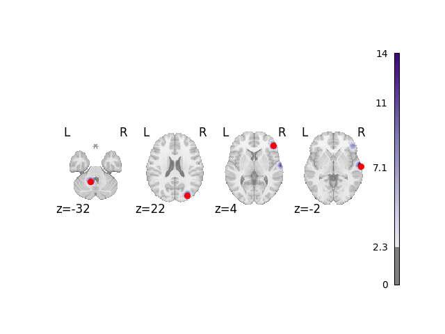
Analyze and plot simple dataset
The red dots in this plot and subsequent plots represent the simulated ground truth foci, and the clouds represent the statistical maps of the simulated data.
analyze_and_plot(studyset, ground_truth_foci)
<Figure size 640x480 with 6 Axes>
Fine-tune collection creation
Perhaps you want more control over the studies being generated. you can set:
the specific peak coordinates (i.e.,
foci)the percentage of studies that contain the foci of interest (
foci_percentage)how tightly the study specific foci are selected around the ground truth (i.e.,
fwhm)the sample size for each study (i.e.,
sample_size)the number of noise foci in each study (i.e.,
n_noise_foci)the number of studies (i.e.,
n_studies)
foci = [(0, 0, 0)]
foci_percentage = 1.0
fwhm = 10.0
n_studies = 30
sample_sizes = [30] * n_studies
sample_sizes[0] = 300
n_noise_foci = 10

_, manual_studyset = create_coordinate_studyset(
    foci=foci, fwhm=fwhm, sample_size=sample_sizes, n_studies=n_studies, n_noise_foci=n_noise_foci
)
Analyze and plot manual dataset
fig = analyze_and_plot(manual_studyset, ground_truth_foci)
fig.show()
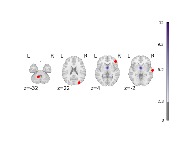
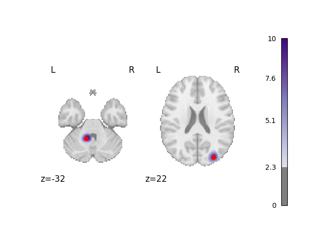
Control percentage of studies with the foci of interest
Often times a converging peak is not found in all studies within the meta-analysis, but only a portion. We can select a percentage of studies where a coordinate is selected around the ground truth foci.
_, perc_foci_studyset = create_coordinate_studyset(
    foci=ground_truth_foci[0:2], foci_percentage="50%", fwhm=10.0, sample_size=30, n_studies=30
)
Analyze and plot the 50% foci dataset
fig = analyze_and_plot(perc_foci_studyset, ground_truth_foci[0:2])
fig.show()
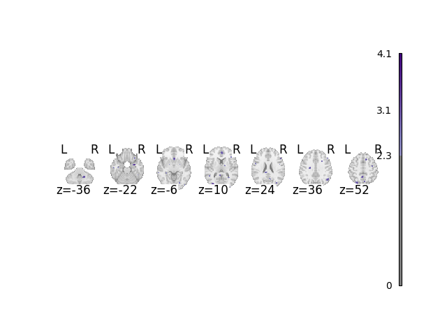
Create a null collection
Perhaps you are interested in the number of false positives your favorite meta-analysis algorithm typically gives. At an alpha of 0.05 we would expect no more than 5% of results to be false positives. To test this, we can create a dataset with no foci that converge, but have many distributed foci.
_, no_foci_studyset = create_coordinate_studyset(
    foci=0, sample_size=(20, 30), n_studies=30, n_noise_foci=100
)
Analyze and plot no foci dataset
When not performing a multiple comparisons correction, there is a false positive rate of approximately 5%.
fig, cres = analyze_and_plot(no_foci_studyset, correct=False, return_cres=True)
fig.show()

p_values = cres.get_map("p", return_type="array")
# what percentage of voxels are not significant?
non_significant_percent = ((p_values > 0.05).sum() / p_values.size) * 100
print(f"{non_significant_percent}% of voxels are not significant")
94.33480827895292% of voxels are not significant
Total running time of the script: (0 minutes 7.879 seconds)