Two-sample ALE meta-analysis

Meta-analytic projects often involve a number of common steps comparing two or more samples.

In this example, we replicate the ALE-based analyses from Enge et al.[1].

A common project workflow with two meta-analytic samples involves the following:

1. Run a within-sample meta-analysis of the first sample.

2. Characterize/summarize the results of the first meta-analysis.

3. Run a within-sample meta-analysis of the second sample.

4. Characterize/summarize the results of the second meta-analysis.

5. Compare the two samples with a subtraction analysis.

6. Compare the two within-sample meta-analyses with a conjunction analysis.

import os
from pathlib import Path

import matplotlib.pyplot as plt
from nilearn.plotting import plot_stat_map

Load Sleuth text files directly into Studysets

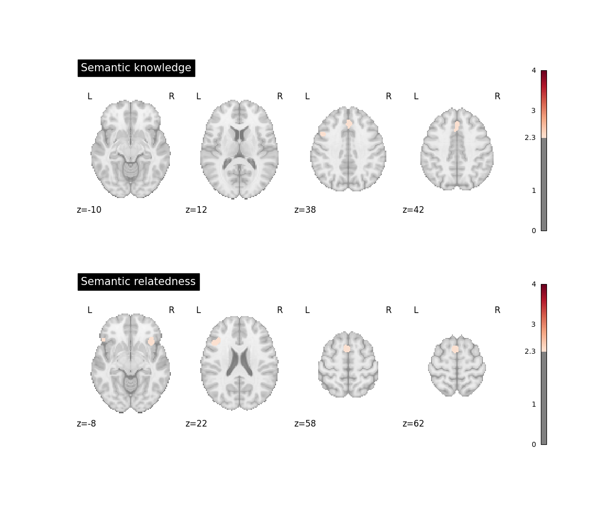
The data for this example are a subset of studies from a meta-analysis on semantic cognition in children [1]. A first group of studies probed children’s semantic world knowledge (e.g., correctly naming an object after hearing its auditory description) while a second group of studies asked children to decide if two (or more) words were semantically related to one another or not.

from nimare.io import convert_sleuth_to_studyset
from nimare.utils import get_resource_path

knowledge_file = os.path.join(get_resource_path(), "semantic_knowledge_children.txt")
related_file = os.path.join(get_resource_path(), "semantic_relatedness_children.txt")

knowledge_studyset = convert_sleuth_to_studyset(knowledge_file)
related_studyset = convert_sleuth_to_studyset(related_file)

Individual group ALEs

Computing separate ALE analyses for each group is not strictly necessary for performing the subtraction analysis but will help the experimenter to appreciate the similarities and differences between the groups.

from nimare.correct import FWECorrector
from nimare.meta.cbma import ALE

ale = ALE(null_method="approximate")
knowledge_results = ale.fit(knowledge_studyset)
related_results = ale.fit(related_studyset)

corr = FWECorrector(method="montecarlo", voxel_thresh=0.001, n_iters=100, n_cores=2)
knowledge_corrected_results = corr.transform(knowledge_results)
related_corrected_results = corr.transform(related_results)

fig, axes = plt.subplots(figsize=(12, 10), nrows=2)
knowledge_img = knowledge_corrected_results.get_map(
    "z_desc-size_level-cluster_corr-FWE_method-montecarlo"
)
plot_stat_map(
    knowledge_img,
    cut_coords=4,
    display_mode="z",
    title="Semantic knowledge",
    threshold=2.326,  # cluster-level p < .01, one-tailed
    cmap="RdBu_r",
    symmetric_cbar=True,
    vmax=4,
    axes=axes[0],
    figure=fig,
)

related_img = related_corrected_results.get_map(
    "z_desc-size_level-cluster_corr-FWE_method-montecarlo"
)
plot_stat_map(
    related_img,
    cut_coords=4,
    display_mode="z",
    title="Semantic relatedness",
    threshold=2.326,  # cluster-level p < .01, one-tailed
    cmap="RdBu_r",
    symmetric_cbar=True,
    vmax=4,
    axes=axes[1],
    figure=fig,
)
fig.show()

  0%|          | 0/100 [00:00<?, ?it/s]
  3%|▎         | 3/100 [00:00<00:04, 23.74it/s]
  7%|▋         | 7/100 [00:00<00:02, 31.06it/s]
 11%|█         | 11/100 [00:00<00:02, 33.99it/s]
 15%|█▌        | 15/100 [00:00<00:02, 35.33it/s]
 19%|█▉        | 19/100 [00:00<00:02, 36.74it/s]
 23%|██▎       | 23/100 [00:00<00:02, 36.34it/s]
 27%|██▋       | 27/100 [00:00<00:02, 36.48it/s]
 31%|███       | 31/100 [00:00<00:01, 37.14it/s]
 35%|███▌      | 35/100 [00:00<00:01, 36.46it/s]
 39%|███▉      | 39/100 [00:01<00:01, 37.09it/s]
 43%|████▎     | 43/100 [00:01<00:01, 37.46it/s]
 47%|████▋     | 47/100 [00:01<00:01, 36.91it/s]
 51%|█████     | 51/100 [00:01<00:01, 37.52it/s]
 55%|█████▌    | 55/100 [00:01<00:01, 36.71it/s]
 59%|█████▉    | 59/100 [00:01<00:01, 37.26it/s]
 63%|██████▎   | 63/100 [00:01<00:01, 36.49it/s]
 67%|██████▋   | 67/100 [00:01<00:00, 37.19it/s]
 71%|███████   | 71/100 [00:01<00:00, 37.69it/s]
 75%|███████▌  | 75/100 [00:02<00:00, 36.78it/s]
 79%|███████▉  | 79/100 [00:02<00:00, 37.42it/s]
 83%|████████▎ | 83/100 [00:02<00:00, 37.70it/s]
 87%|████████▋ | 87/100 [00:02<00:00, 36.86it/s]
 91%|█████████ | 91/100 [00:02<00:00, 37.18it/s]
 95%|█████████▌| 95/100 [00:02<00:00, 37.73it/s]
 99%|█████████▉| 99/100 [00:02<00:00, 37.05it/s]
100%|██████████| 100/100 [00:02<00:00, 36.97it/s]

  0%|          | 0/100 [00:00<?, ?it/s]
  3%|▎         | 3/100 [00:00<00:03, 29.11it/s]
  9%|▉         | 9/100 [00:00<00:02, 38.45it/s]
 13%|█▎        | 13/100 [00:00<00:02, 38.70it/s]
 19%|█▉        | 19/100 [00:00<00:02, 40.22it/s]
 25%|██▌       | 25/100 [00:00<00:01, 40.78it/s]
 31%|███       | 31/100 [00:00<00:01, 42.28it/s]
 36%|███▌      | 36/100 [00:00<00:01, 44.08it/s]
 41%|████      | 41/100 [00:01<00:01, 40.45it/s]
 46%|████▌     | 46/100 [00:01<00:01, 42.15it/s]
 51%|█████     | 51/100 [00:01<00:01, 40.36it/s]
 56%|█████▌    | 56/100 [00:01<00:01, 42.23it/s]
 61%|██████    | 61/100 [00:01<00:00, 39.76it/s]
 67%|██████▋   | 67/100 [00:01<00:00, 41.05it/s]
 73%|███████▎  | 73/100 [00:01<00:00, 41.23it/s]
 79%|███████▉  | 79/100 [00:01<00:00, 41.19it/s]
 85%|████████▌ | 85/100 [00:02<00:00, 41.26it/s]
 91%|█████████ | 91/100 [00:02<00:00, 42.46it/s]
 96%|█████████▌| 96/100 [00:02<00:00, 43.80it/s]
100%|██████████| 100/100 [00:02<00:00, 41.56it/s]

Characterize the relative contributions of experiments in the ALE results

NiMARE contains two methods for this: Jackknife and FocusCounter. We will show both below, but for the sake of speed we will only apply one to each subgroup meta-analysis.

from nimare.diagnostics import FocusCounter

counter = FocusCounter(
    target_image="z_desc-size_level-cluster_corr-FWE_method-montecarlo",
    voxel_thresh=None,
)
knowledge_diagnostic_results = counter.transform(knowledge_corrected_results)

  0%|          | 0/21 [00:00<?, ?it/s]
 24%|██▍       | 5/21 [00:00<00:00, 49.15it/s]
 48%|████▊     | 10/21 [00:00<00:00, 49.35it/s]
 71%|███████▏  | 15/21 [00:00<00:00, 49.38it/s]
 95%|█████████▌| 20/21 [00:00<00:00, 49.36it/s]
100%|██████████| 21/21 [00:00<00:00, 49.33it/s]

Clusters table.

knowledge_clusters_table = knowledge_diagnostic_results.tables[
    "z_desc-size_level-cluster_corr-FWE_method-montecarlo_tab-clust"
]
knowledge_clusters_table.head(10)

	Cluster ID	X	Y	Z	Peak Stat	Cluster Size (mm3)
0	PositiveTail 1	36.0	24.0	-6.0	2.326348	1128
1	PositiveTail 2	-2.0	20.0	46.0	2.326348	3472
2	PositiveTail 3	-44.0	12.0	30.0	2.326348	3096
3	PositiveTail 4	-34.0	22.0	0.0	2.326348	992
4	PositiveTail 5	-52.0	-38.0	4.0	1.405072	672
5	PositiveTail 6	54.0	-28.0	4.0	0.877896	512
6	PositiveTail 7	-6.0	-14.0	12.0	0.877896	512

Contribution table. Here PostiveTail refers to clusters with positive statistics.

knowledge_count_table = knowledge_diagnostic_results.tables[
    "z_desc-size_level-cluster_corr-FWE_method-montecarlo_diag-FocusCounter"
    "_tab-counts_tail-positive"
]
knowledge_count_table.head(10)

	id	PositiveTail 1	PositiveTail 2	PositiveTail 3	PositiveTail 4	PositiveTail 5	PositiveTail 6	PositiveTail 7
0	arnoldussen2006nc-analysis_1	0	0	1	0	0	0	0
1	arnoldussen2006rm-analysis_1	0	0	1	0	0	0	0
2	backes2002-analysis_1	0	1	1	0	0	0	0
3	balsamo2002-analysis_1	0	0	0	0	1	0	0
4	balsamo2006-analysis_1	0	1	1	0	0	0	0
5	bauer2017-analysis_1	1	0	0	0	0	0	1
6	berl2014-analysis_1	1	2	2	0	0	1	1
7	brauer2007-analysis_1	0	1	0	0	0	0	0
8	gaillard2001-analysis_1	0	0	1	0	0	0	0
9	gaillard2003-analysis_1	1	1	1	0	0	0	0

from nimare.diagnostics import Jackknife

jackknife = Jackknife(
    target_image="z_desc-size_level-cluster_corr-FWE_method-montecarlo",
    voxel_thresh=None,
)
related_diagnostic_results = jackknife.transform(related_corrected_results)
related_jackknife_table = related_diagnostic_results.tables[
    "z_desc-size_level-cluster_corr-FWE_method-montecarlo_diag-Jackknife_tab-counts_tail-positive"
]
related_jackknife_table.head(10)

  0%|          | 0/16 [00:00<?, ?it/s]
  6%|▋         | 1/16 [00:00<00:02,  6.99it/s]
 12%|█▎        | 2/16 [00:00<00:02,  6.98it/s]
 19%|█▉        | 3/16 [00:00<00:01,  6.98it/s]
 25%|██▌       | 4/16 [00:00<00:01,  6.97it/s]
 31%|███▏      | 5/16 [00:00<00:01,  7.00it/s]
 38%|███▊      | 6/16 [00:00<00:01,  6.96it/s]
 44%|████▍     | 7/16 [00:01<00:01,  6.97it/s]
 50%|█████     | 8/16 [00:01<00:01,  6.97it/s]
 56%|█████▋    | 9/16 [00:01<00:01,  6.96it/s]
 62%|██████▎   | 10/16 [00:01<00:00,  6.97it/s]
 69%|██████▉   | 11/16 [00:01<00:00,  6.97it/s]
 75%|███████▌  | 12/16 [00:01<00:00,  6.98it/s]
 81%|████████▏ | 13/16 [00:01<00:00,  6.98it/s]
 88%|████████▊ | 14/16 [00:02<00:00,  6.98it/s]
 94%|█████████▍| 15/16 [00:02<00:00,  7.00it/s]
100%|██████████| 16/16 [00:02<00:00,  7.02it/s]
100%|██████████| 16/16 [00:02<00:00,  6.98it/s]

	id	PositiveTail 1	PositiveTail 2	PositiveTail 3	PositiveTail 4	PositiveTail 5
0	booth2001-analysis_1	0.0	0.0	0.029415	0.054821	0.0
1	booth2003-analysis_1	0.0	0.0	0.0	0.000008	0.0
2	booth2007-analysis_1	0.021799	0.068333	0.051598	0.000028	0.000019
3	cao2008-analysis_1	0.134026	0.06561	0.035607	0.094222	0.0
4	chou2006a-analysis_1	0.211268	0.123099	0.000075	0.095687	0.0
5	chou2006b-analysis_1	0.21024	0.117018	0.004724	0.117981	0.0
6	chou2009-analysis_1	0.188491	0.1575	0.22325	0.212472	0.330668
7	chou2019-analysis_1	0.0	0.061734	0.0	0.0	0.0
8	fan2020-analysis_1	0.0	0.070051	0.002654	0.101595	0.0
9	lee2011aud-analysis_1	0.000026	0.000246	0.164283	0.068827	0.243831

Subtraction analysis

Typically, one would use at least 5000 iterations for a subtraction analysis. However, we have reduced this to 100 iterations for this example. Here we use a cluster-defining p-threshold of 0.01 for Monte Carlo FWE correction. In practice one would generally use a more stringent threshold.

from nimare.meta.cbma import ALESubtraction
from nimare.reports.base import run_reports
from nimare.workflows import PairwiseCBMAWorkflow

subtraction_iters = 100
subtraction_voxel_thresh = 0.01

# Keep estimator and Corrector Monte Carlo parameters synchronized so the
# correction step can reuse cached permutation nulls from ALESubtraction.
subtraction_estimator = ALESubtraction(
    n_iters=subtraction_iters,
    voxel_thresh=subtraction_voxel_thresh,
    vfwe_only=False,
    n_cores=1,
)
subtraction_corrector = FWECorrector(
    method="montecarlo",
    voxel_thresh=subtraction_voxel_thresh,
    n_iters=subtraction_iters,
    n_cores=1,
    vfwe_only=False,
)

workflow = PairwiseCBMAWorkflow(
    estimator=subtraction_estimator,
    corrector=subtraction_corrector,
    diagnostics=FocusCounter(voxel_thresh=0.01, display_second_group=True),
)
res_sub = workflow.fit(knowledge_studyset, related_studyset)

  0%|          | 0/100 [00:00<?, ?it/s]
 17%|█▋        | 17/100 [00:00<00:00, 167.69it/s]
 34%|███▍      | 34/100 [00:00<00:00, 168.32it/s]
 51%|█████     | 51/100 [00:00<00:00, 167.99it/s]
 68%|██████▊   | 68/100 [00:00<00:00, 166.15it/s]
 85%|████████▌ | 85/100 [00:00<00:00, 166.12it/s]
100%|██████████| 100/100 [00:00<00:00, 166.87it/s]
/home/docs/checkouts/readthedocs.org/user_builds/nimare/checkouts/latest/nimare/diagnostics.py:324: UserWarning: Attention: At least one of the (sub)peaks falls outside of the cluster body. Identifying the nearest in-cluster voxel.
  clusters_table, label_maps = get_clusters_table(

  0%|          | 0/21 [00:00<?, ?it/s]
  5%|▍         | 1/21 [00:00<00:15,  1.26it/s]
 10%|▉         | 2/21 [00:01<00:15,  1.26it/s]
 14%|█▍        | 3/21 [00:02<00:14,  1.26it/s]
 19%|█▉        | 4/21 [00:03<00:13,  1.26it/s]
 24%|██▍       | 5/21 [00:03<00:12,  1.26it/s]
 29%|██▊       | 6/21 [00:04<00:11,  1.26it/s]
 33%|███▎      | 7/21 [00:05<00:11,  1.26it/s]
 38%|███▊      | 8/21 [00:06<00:10,  1.25it/s]
 43%|████▎     | 9/21 [00:07<00:09,  1.26it/s]
 48%|████▊     | 10/21 [00:07<00:08,  1.26it/s]
 52%|█████▏    | 11/21 [00:08<00:07,  1.25it/s]
 57%|█████▋    | 12/21 [00:09<00:07,  1.26it/s]
 62%|██████▏   | 13/21 [00:10<00:06,  1.26it/s]
 67%|██████▋   | 14/21 [00:11<00:05,  1.26it/s]
 71%|███████▏  | 15/21 [00:11<00:04,  1.26it/s]
 76%|███████▌  | 16/21 [00:12<00:03,  1.26it/s]
 81%|████████  | 17/21 [00:13<00:03,  1.26it/s]
 86%|████████▌ | 18/21 [00:14<00:02,  1.26it/s]
 90%|█████████ | 19/21 [00:15<00:01,  1.26it/s]
 95%|█████████▌| 20/21 [00:15<00:00,  1.26it/s]
100%|██████████| 21/21 [00:16<00:00,  1.26it/s]
100%|██████████| 21/21 [00:16<00:00,  1.26it/s]

  0%|          | 0/16 [00:00<?, ?it/s]
  6%|▋         | 1/16 [00:00<00:13,  1.14it/s]
 12%|█▎        | 2/16 [00:01<00:12,  1.14it/s]
 19%|█▉        | 3/16 [00:02<00:11,  1.14it/s]
 25%|██▌       | 4/16 [00:03<00:10,  1.14it/s]
 31%|███▏      | 5/16 [00:04<00:09,  1.14it/s]
 38%|███▊      | 6/16 [00:05<00:08,  1.13it/s]
 44%|████▍     | 7/16 [00:06<00:07,  1.13it/s]
 50%|█████     | 8/16 [00:07<00:07,  1.14it/s]
 56%|█████▋    | 9/16 [00:07<00:06,  1.14it/s]
 62%|██████▎   | 10/16 [00:08<00:05,  1.14it/s]
 69%|██████▉   | 11/16 [00:09<00:04,  1.13it/s]
 75%|███████▌  | 12/16 [00:10<00:03,  1.14it/s]
 81%|████████▏ | 13/16 [00:11<00:02,  1.14it/s]
 88%|████████▊ | 14/16 [00:12<00:01,  1.14it/s]
 94%|█████████▍| 15/16 [00:13<00:00,  1.14it/s]
100%|██████████| 16/16 [00:14<00:00,  1.13it/s]
100%|██████████| 16/16 [00:14<00:00,  1.14it/s]

Report

Finally, a NiMARE report is generated from the MetaResult. root_dir = Path(os.getcwd()).parents[1] / “docs” / “_build” Use the previous root to run the documentation locally.

root_dir = Path(os.getcwd()).parents[1] / "_readthedocs"
html_dir = root_dir / "html" / "auto_examples" / "02_meta-analyses" / "08_subtraction"
html_dir.mkdir(parents=True, exist_ok=True)

run_reports(res_sub, html_dir)

Conjunction analysis

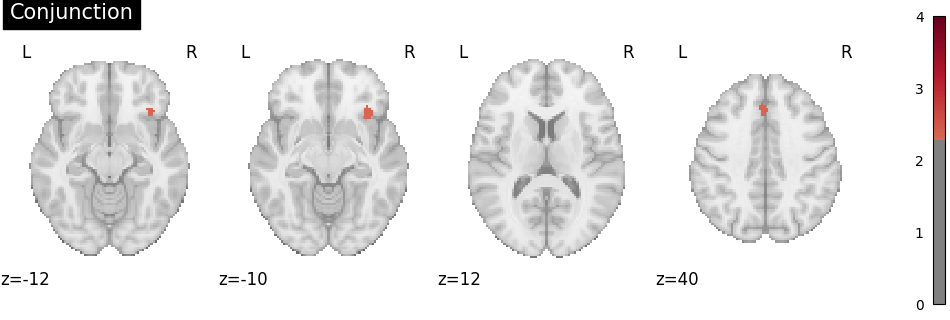
To determine the overlap of the meta-analytic results, a conjunction image can be computed by (a) identifying voxels that were statistically significant in both individual group maps and (b) selecting, for each of these voxels, the smaller of the two group-specific z values Nichols et al.[2].

from nimare.workflows.misc import conjunction_analysis

img_conj = conjunction_analysis([knowledge_img, related_img])

plot_stat_map(
    img_conj,
    cut_coords=4,
    display_mode="z",
    title="Conjunction",
    threshold=2.326,  # cluster-level p < .01, one-tailed
    cmap="RdBu_r",
    symmetric_cbar=True,
    vmax=4,
)

<nilearn.plotting.displays._slicers.ZSlicer object at 0x78fa391abbf0>

References

[1] (1,2)

Alexander Enge, Rasha Abdel Rahman, and Michael A Skeide. A meta-analysis of fmri studies of semantic cognition in children. NeuroImage, 241:118436, 2021. URL: https://doi.org/10.1016/j.neuroimage.2021.118436, doi:10.1016/j.neuroimage.2021.118436.

[2]

Thomas Nichols, Matthew Brett, Jesper Andersson, Tor Wager, and Jean-Baptiste Poline. Valid conjunction inference with the minimum statistic. Neuroimage, 25(3):653–660, 2005. URL: https://doi.org/10.1016/j.neuroimage.2004.12.005, doi:10.1016/j.neuroimage.2004.12.005.