The Estimator class

An introduction to the Estimator class.

The Estimator class is the base for all meta-analyses in NiMARE. A general rule of thumb for Estimators is that they ingest Datasets and output MetaResult objects.

Start with the necessary imports

import os

Load Dataset

from nimare.dataset import Dataset
from nimare.utils import get_resource_path

dset_file = os.path.join(get_resource_path(), "nidm_pain_dset.json")
dset = Dataset(dset_file)

# We will reduce the Dataset to the first 10 studies
dset = dset.slice(dset.ids[:10])

The Estimator

from pprint import pprint

from nimare.meta.cbma.ale import ALE

# First, the Estimator should be initialized with any parameters.
meta = ALE()

# Then, the ``fit`` method takes in the Dataset and produces a MetaResult.
results = meta.fit(dset)

# You can also look at the description of the Estimator.
print("Description:")
pprint(results.description_)
print("References:")
pprint(results.bibtex_)

Description:
('An activation likelihood estimation (ALE) meta-analysis '
 '\\citep{turkeltaub2002meta,turkeltaub2012minimizing,eickhoff2012activation} '
 'was performed with NiMARE 0.2.2+2.gbf7df33.dirty (RRID:SCR_017398; '
 '\\citealt{Salo2023}), using a(n) ALE kernel. An ALE kernel '
 '\\citep{eickhoff2012activation} was used to generate study-wise modeled '
 'activation maps from coordinates. In this kernel method, each coordinate is '
 'convolved with a Gaussian kernel with full-width at half max values '
 'determined on a study-wise basis based on the study sample sizes according '
 'to the formulae provided in \\cite{eickhoff2012activation}. For voxels with '
 'overlapping kernels, the maximum value was retained. ALE values were '
 'converted to p-values using an approximate null distribution '
 '\\citep{eickhoff2012activation}. The input dataset included 147 foci from 10 '
 'experiments, with a total of 153 participants.')
References:
('@article{Salo2023,\n'
 '  doi = {10.52294/001c.87681},\n'
 '  url = {https://doi.org/10.52294/001c.87681},\n'
 '  year = {2023},\n'
 '  volume = {3},\n'
 '  pages = {1 - 32},\n'
 '  author = {Taylor Salo and Tal Yarkoni and Thomas E. Nichols and '
 'Jean-Baptiste Poline and Murat Bilgel and Katherine L. Bottenhorn and Dorota '
 'Jarecka and James D. Kent and Adam Kimbler and Dylan M. Nielson and Kendra '
 'M. Oudyk and Julio A. Peraza and Alexandre Pérez and Puck C. Reeders and '
 'Julio A. Yanes and Angela R. Laird},\n'
 '  title = {NiMARE: Neuroimaging Meta-Analysis Research Environment},\n'
 '  journal = {Aperture Neuro}\n'
 '}\n'
 '@article{eickhoff2012activation,\n'
 '  title={Activation likelihood estimation meta-analysis revisited},\n'
 '  author={Eickhoff, Simon B and Bzdok, Danilo and Laird, Angela R and Kurth, '
 'Florian and Fox, Peter T},\n'
 '  journal={Neuroimage},\n'
 '  volume={59},\n'
 '  number={3},\n'
 '  pages={2349--2361},\n'
 '  year={2012},\n'
 '  publisher={Elsevier},\n'
 '  url={https://doi.org/10.1016/j.neuroimage.2011.09.017},\n'
 '  doi={10.1016/j.neuroimage.2011.09.017}\n'
 '}\n'
 '@article{turkeltaub2002meta,\n'
 '  title={Meta-analysis of the functional neuroanatomy of single-word '
 'reading: method and validation},\n'
 '  author={Turkeltaub, Peter E and Eden, Guinevere F and Jones, Karen M and '
 'Zeffiro, Thomas A},\n'
 '  journal={Neuroimage},\n'
 '  volume={16},\n'
 '  number={3},\n'
 '  pages={765--780},\n'
 '  year={2002},\n'
 '  publisher={Elsevier},\n'
 '  url={https://doi.org/10.1006/nimg.2002.1131},\n'
 '  doi={10.1006/nimg.2002.1131}\n'
 '}\n'
 '@article{turkeltaub2012minimizing,\n'
 '  title={Minimizing within-experiment and within-group effects in activation '
 'likelihood estimation meta-analyses},\n'
 '  author={Turkeltaub, Peter E and Eickhoff, Simon B and Laird, Angela R and '
 'Fox, Mick and Wiener, Martin and Fox, Peter},\n'
 '  journal={Human brain mapping},\n'
 '  volume={33},\n'
 '  number={1},\n'
 '  pages={1--13},\n'
 '  year={2012},\n'
 '  publisher={Wiley Online Library},\n'
 '  url={https://doi.org/10.1002/hbm.21186},\n'
 '  doi={10.1002/hbm.21186}\n'
 '}')

Coordinate-based Estimators allow you to provide a specific KernelTransformer

Each CBMA Estimator’s default KernelTransformer will always be the most appropriate type for that algorithm, but you can swap out the kernel as you wish.

For example, an ALE Estimator could be initialized with an MKDAKernel, though there is no guarantee that the results would make sense.

from nimare.meta.kernel import MKDAKernel

meta = ALE(kernel_transformer=MKDAKernel)
results = meta.fit(dset)

from nilearn.plotting import plot_stat_map

plot_stat_map(results.get_map("z"), draw_cross=False, cmap="RdBu_r")

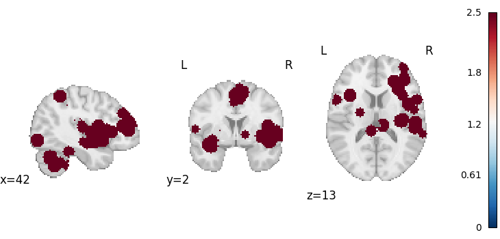
<nilearn.plotting.displays._slicers.OrthoSlicer object at 0x7fe923215370>

CBMA Estimators can accept KernelTransformers a few different ways

from nimare.meta.kernel import ALEKernel

Initializing the Estimator with a KernelTransformer class alone will use its default settings.

meta = ALE(kernel_transformer=ALEKernel)
print(meta.kernel_transformer)

ALEKernel(memory=Memory(location=None))

You can also initialize the Estimator with an initialized KernelTransformer object.

kernel = ALEKernel()
meta = ALE(kernel_transformer=kernel)
print(meta.kernel_transformer)

ALEKernel()

This is especially useful if you want to initialize the KernelTransformer with parameters with non-default values.

kernel = ALEKernel(sample_size=20)
meta = ALE(kernel_transformer=kernel)
print(meta.kernel_transformer)

ALEKernel(sample_size=20)

You can also provide specific initialization values to the KernelTransformer via the Estimator, by including keyword arguments starting with kernel__.

meta = ALE(kernel__sample_size=20)
print(meta.kernel_transformer)

ALEKernel(memory=Memory(location=None), sample_size=20)

Most CBMA Estimators have multiple ways to test uncorrected statistical significance

For most Estimators, the two options, defined with the null_method parameter, are "approximate" and "montecarlo". For more information about these options, see Null methods.

meta = ALE(null_method="approximate")
results = meta.fit(dset)

Note that, to measure significance appropriately with the montecarlo method, you need a lot more than 10 iterations. We recommend 5000 (the default value).

mc_meta = ALE(null_method="montecarlo", n_iters=10, n_cores=1)
mc_results = mc_meta.fit(dset)

  0%|          | 0/10 [00:00<?, ?it/s]
 10%|█         | 1/10 [00:00<00:02,  3.84it/s]
 20%|██        | 2/10 [00:00<00:02,  3.85it/s]
 30%|███       | 3/10 [00:00<00:01,  3.88it/s]
 40%|████      | 4/10 [00:01<00:01,  3.89it/s]
 50%|█████     | 5/10 [00:01<00:01,  3.88it/s]
 60%|██████    | 6/10 [00:01<00:01,  3.89it/s]
 70%|███████   | 7/10 [00:01<00:00,  3.91it/s]
 80%|████████  | 8/10 [00:02<00:00,  3.92it/s]
 90%|█████████ | 9/10 [00:02<00:00,  3.89it/s]
100%|██████████| 10/10 [00:02<00:00,  3.89it/s]
100%|██████████| 10/10 [00:02<00:00,  3.89it/s]

The null distributions are stored within the Estimators

pprint(meta.null_distributions_)

{'histogram_bins': array([0.000e+00, 1.000e-05, 2.000e-05, ..., 7.247e-02, 7.248e-02,
       7.249e-02]),
 'histweights_corr-none_method-approximate': array([5.17138782e-01, 1.68074450e-21, 5.51924442e-02, ...,
       0.00000000e+00, 0.00000000e+00, 0.00000000e+00])}

As well as the MetaResult, which stores a copy of the Estimator

pprint(results.estimator.null_distributions_)

{'histogram_bins': array([0.000e+00, 1.000e-05, 2.000e-05, ..., 7.247e-02, 7.248e-02,
       7.249e-02]),
 'histweights_corr-none_method-approximate': array([5.17138782e-01, 1.68074450e-21, 5.51924442e-02, ...,
       0.00000000e+00, 0.00000000e+00, 0.00000000e+00])}

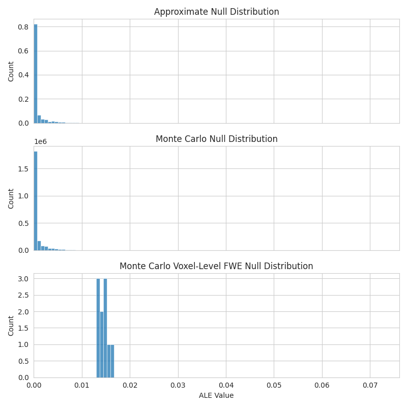
The null distributions also differ based on the null method. For example, the "montecarlo" option creates a histweights_corr-none_method-montecarlo distribution, instead of the histweights_corr-none_method-approximate produced by the "approximate" method.

pprint(mc_meta.null_distributions_)

{'histogram_bins': array([0.000e+00, 1.000e-05, 2.000e-05, ..., 7.247e-02, 7.248e-02,
       7.249e-02]),
 'histweights_corr-none_method-montecarlo': array([872425, 122765,  83437, ...,      0,      0,      0]),
 'histweights_level-voxel_corr-fwe_method-montecarlo': array([0, 0, 0, ..., 0, 0, 0])}

import matplotlib.pyplot as plt
import seaborn as sns

with sns.axes_style("whitegrid"):
    fig, axes = plt.subplots(figsize=(8, 8), sharex=True, nrows=3)
    sns.histplot(
        x=meta.null_distributions_["histogram_bins"],
        weights=meta.null_distributions_["histweights_corr-none_method-approximate"],
        bins=100,
        ax=axes[0],
    )
    axes[0].set_xlim(0, None)
    axes[0].set_title("Approximate Null Distribution")
    sns.histplot(
        x=mc_meta.null_distributions_["histogram_bins"],
        weights=mc_meta.null_distributions_["histweights_corr-none_method-montecarlo"],
        bins=100,
        ax=axes[1],
    )
    axes[1].set_title("Monte Carlo Null Distribution")
    sns.histplot(
        x=mc_meta.null_distributions_["histogram_bins"],
        weights=mc_meta.null_distributions_["histweights_level-voxel_corr-fwe_method-montecarlo"],
        bins=100,
        ax=axes[2],
    )
    axes[2].set_title("Monte Carlo Voxel-Level FWE Null Distribution")
    axes[2].set_xlabel("ALE Value")
    fig.tight_layout()