Coordinate-based meta-regression with a model formula

A tour of coordinate-based meta-regression (CBMR) in NiMARE.

CBMR estimates a smooth activation-intensity function from reported coordinates. The model is written as a formula, in which every term states its own spatial resolution:

CBMR("~ s(diagnosis) + sample_size")

Use s(term) when the effect of term should vary across the brain. s(diagnosis) gives each diagnosis level a smooth spatial map, s(diagnosis:drug_status) gives each level combination its own map, and s(standardized_avg_age) estimates an age-effect map. Without s(), a term gets a single coefficient that applies to the whole brain. Because each term declares this separately, a model can freely mix scalar and spatial effects.

The parameter cost follows from the same mark. At spline_spacing=10 on the 2 mm brain mask the basis has 457 columns, so every s() term costs 457 coefficients per column – as much as another group’s entire baseline map. That is worth knowing before adding one, which is why the budget is logged at fit time and available from describe_terms().

For more background on model formulas, Patsy’s formula documentation introduces the notation used by Python model libraries, and R’s formula documentation gives the broader Wilkinson-style conventions. NiMARE’s s() term is inspired by mgcv’s smooth-term syntax.

import matplotlib.pyplot as plt
import numpy as np
from nilearn.plotting import plot_stat_map

from nimare.correct import FDRCorrector
from nimare.generate import create_coordinate_studyset
from nimare.meta.cbmr import CBMR
from nimare.transforms import StandardizeField

Simulate a Studyset

A coordinate-based Studyset with reported foci, sample sizes, diagnosis and drug-status labels, and two continuous moderators. Coarse B-spline spacing keeps the example quick; a real analysis would use spline_spacing of 10 or 5.

_, studyset = create_coordinate_studyset(
    foci=10,
    sample_size=(20, 40),
    n_studies=200,
    seed=100,
)

annotations_df = studyset.annotations_df.copy()
n_rows = annotations_df.shape[0]
group_pattern = [
    ("schizophrenia", "Yes"),
    ("schizophrenia", "No"),
    ("depression", "Yes"),
    ("depression", "No"),
]
annotations_df[["diagnosis", "drug_status"]] = [
    group_pattern[i % len(group_pattern)] for i in range(n_rows)
]
annotations_df["sample_sizes"] = [studyset.metadata.sample_sizes[i][0] for i in range(n_rows)]
annotations_df["avg_age"] = np.arange(n_rows)
# A Studyset is immutable, so the edited frame is attached to a new one rather than assigned back.
studyset = studyset.with_annotations_df(annotations_df, name="moderators", replace=True)

studyset = StandardizeField(fields=["sample_sizes", "avg_age"]).transform(studyset)

FIT_KWARGS = dict(
    spline_spacing=100,  # a reasonable analysis choice is 10 or 5; 100 is for speed
    n_iter=200,
    lr=1e-1,
    tol=1e3,  # a reasonable analysis choice is 1e-2; 1e3 is for speed
    device="cpu",  # use "cuda" if you have a GPU
    random_state=100,
)

One spatial map per group

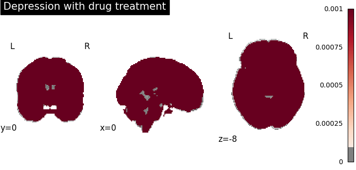
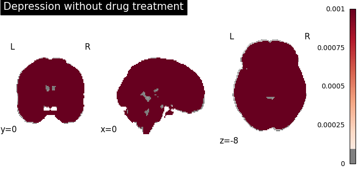
s(diagnosis:drug_status) crosses the two factors and gives every combination of levels its own intensity map. This is the model the old group_categories=["diagnosis", "drug_status"] argument produced – note that it was always a full interaction, which the formula now says out loud.

group_results = CBMR("~ s(diagnosis:drug_status)", **FIT_KWARGS).fit(dataset=studyset)

print(group_results.describe_terms())

plot_stat_map(
    group_results.get_map("spatialIntensity_group-schizophrenia-Yes"),
    cut_coords=[0, 0, -8],
    draw_cross=False,
    cmap="RdBu_r",
    symmetric_cbar=True,
    title="Schizophrenia, on drug treatment",
    threshold=1e-4,
    vmax=1e-3,
)
plot_stat_map(
    group_results.get_map("spatialIntensity_group-depression-No"),
    cut_coords=[0, 0, -8],
    draw_cross=False,
    cmap="RdBu_r",
    symmetric_cbar=True,
    title="Depression, no drug treatment",
    threshold=1e-4,
    vmax=1e-3,
)

• 
• 

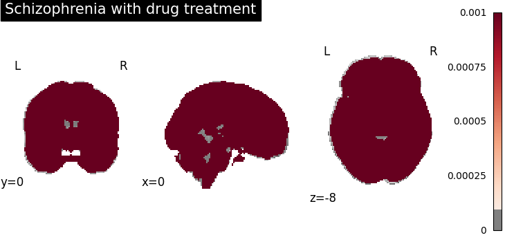
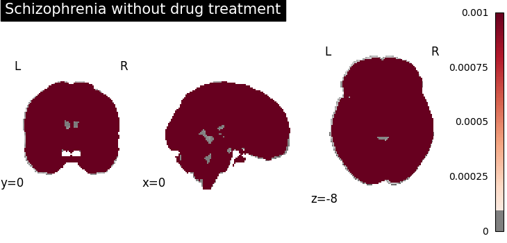
  s(diagnosis:drug_status)            4 column(s) x    15 =      60 parameters
  total                                                       60

<nilearn.plotting.displays._slicers.OrthoSlicer object at 0x7af10ff4ad00>

Testing hypotheses by name

Hypotheses are written over the levels of a term, in the same notation the map keys use. This replaces passing contrast matrices positionally, which was unreadable and silently depended on level ordering – reorder the levels and the same matrix tested a different hypothesis.

Parsing is patsy.DesignInfo.linear_constraint(), the same parser statsmodels uses for t_test, so arithmetic ("2 * a = b + c"), bare difference expressions ("a - b") and non-zero right-hand sides ("a = 1") all work.

Each contrast reports its effect size and standard error, not only its significance – est_ and se_ alongside z_, p_ and logp_, which is the vocabulary the rest of NiMARE uses.

drug_effect = group_results.test(
    "schizophrenia-Yes = schizophrenia-No",
    name="schizophrenia-drug",
)

plot_stat_map(
    drug_effect.get_map("z_schizophrenia-drug"),
    cut_coords=[0, 0, -8],
    draw_cross=False,
    cmap="RdBu_r",
    symmetric_cbar=True,
    title="Drug effect within schizophrenia",
    threshold=None,
    vmax=2,
)

<nilearn.plotting.displays._slicers.OrthoSlicer object at 0x7af10ff4b800>

The effect size is a map in its own right, and worth looking at before the statistics: a significant contrast whose estimate is negligible is a large sample, not a large effect.

plot_stat_map(
    drug_effect.get_map("est_schizophrenia-drug"),
    cut_coords=[0, 0, -8],
    draw_cross=False,
    cmap="RdBu_r",
    symmetric_cbar=True,
    title="Drug effect: estimate on log intensity",
)

<nilearn.plotting.displays._slicers.OrthoSlicer object at 0x7af1047101b0>

Asking which levels differ is a request for every comparison, so there is no need to write them out one at a time. method= generates a named family, after emmeans’ contrast families and gratia::difference_smooths: "pairwise" for all pairs, "reference" against the first level, "consecutive" against the previous one, "zero" against zero.

all_pairs = group_results.test(term="diagnosis:drug_status", method="pairwise")
print(sorted(name for name in all_pairs.maps if name.startswith("z_")))

['z_depression-No_vs_depression-Yes', 'z_depression-No_vs_schizophrenia-No', 'z_depression-No_vs_schizophrenia-Yes', 'z_depression-Yes_vs_schizophrenia-Yes', 'z_schizophrenia-No_vs_depression-Yes', 'z_schizophrenia-No_vs_schizophrenia-Yes']

A list of statements is tested jointly, as a generalized linear hypothesis, rather than one at a time. This asks whether the drug effect is zero in both diagnoses at once.

joint = group_results.test(
    ["schizophrenia-Yes = schizophrenia-No", "depression-Yes = depression-No"],
    name="drug-anywhere",
)

plot_stat_map(
    joint.get_map("chiSquare_drug-anywhere"),
    cut_coords=[0, 0, -8],
    draw_cross=False,
    cmap="Reds",
    title="Joint test: any drug effect",
)

<nilearn.plotting.displays._slicers.OrthoSlicer object at 0x7af10ff4b490>

Robust standard errors and multiple comparisons

The default standard errors come from the Fisher information, which is correct only if the Poisson mean-variance relationship holds. Foci are overdispersed and correlated within an experiment, so cov_type="sandwich" is usually the safer choice; meat="cluster" allows arbitrary correlation among one experiment’s own foci.

robust = group_results.test(
    "schizophrenia-Yes = schizophrenia-No",
    name="drug-robust",
    cov_type="sandwich",
    meat="cluster",
    correction="hc1",
)

corrected = FDRCorrector(method="indep", alpha=0.05).transform(robust)

plot_stat_map(
    corrected.get_map("z_drug-robust_corr-FDR_method-indep"),
    cut_coords=[0, 0, -8],
    draw_cross=False,
    cmap="RdBu_r",
    symmetric_cbar=True,
    title="Drug effect, clustered SEs, FDR corrected",
    threshold=None,
    vmax=2,
)

<nilearn.plotting.displays._slicers.OrthoSlicer object at 0x7af104710b50>

Moderators, global and spatially varying

Whether a moderator gets one coefficient or a map is decided by s(), per term. Here sample size is allowed only to scale the whole map, while age is allowed to reshape it.

Under the log link a global moderator can only rescale the intensity – it multiplies every voxel by the same factor. A spatially varying one can change the pattern. That is the real distinction, and it is why the two answers arrive in different places: a scalar coefficient in a table, a coefficient map among the maps.

The next fit moves from a model whose moderator effect is global to one that includes a spatially varying covariate. standardized_sample_sizes remains global, while s(standardized_avg_age) estimates an age-effect map, allowing the association with age to differ across voxels.

mixed_results = CBMR(
    "~ s(diagnosis:drug_status) + standardized_sample_sizes + s(standardized_avg_age)",
    **FIT_KWARGS,
).fit(dataset=studyset)

print(mixed_results.describe_terms())
print(mixed_results.tables["moderatorEffect_standardized_sample_sizes"])

plot_stat_map(
    mixed_results.get_map("voxelwiseModeratorEffect_standardized_avg_age"),
    cut_coords=[0, 0, -8],
    draw_cross=False,
    cmap="RdBu_r",
    symmetric_cbar=True,
    title="Age effect on log intensity (per SD)",
)

  s(diagnosis:drug_status)            4 column(s) x    15 =      60 parameters
  standardized_sample_sizes           1 column(s) x     1 =       1 parameters
  s(standardized_avg_age)             1 column(s) x    15 =      15 parameters
  total                                                       76
                      column       est      se
0  standardized_sample_sizes  0.001812  1.1306

<nilearn.plotting.displays._slicers.OrthoSlicer object at 0x7af1047119c0>

Comparing model-based and robust uncertainty

The fitted coefficient map is unchanged by the covariance estimator. What changes is the uncertainty attached to the same spatially varying effect. By default, test uses the inverse Fisher information matrix. Passing cov_type="sandwich" asks for clustered robust standard errors instead, allowing foci from the same experiment to be correlated.

age_model_based = mixed_results.test("standardized_avg_age = 0", name="age-model-based")
age_robust = mixed_results.test(
    "standardized_avg_age = 0",
    name="age-robust",
    cov_type="sandwich",
    meat="cluster",
    correction="hc1",
)

figure, axes = plt.subplots(1, 2, figsize=(10, 4))
for axis, result, map_name, title in (
    (axes[0], age_model_based, "z_age-model-based", "Inverse Fisher information"),
    (axes[1], age_robust, "z_age-robust", "Clustered sandwich"),
):
    plot_stat_map(
        result.get_map(map_name),
        axes=axis,
        cut_coords=[0, 0, -8],
        draw_cross=False,
        cmap="RdBu_r",
        symmetric_cbar=True,
        title=title,
        threshold=1e-6,
        vmax=2,
    )

Reading a moderator map: relative intensity and intensity difference

A moderator’s coefficient map is a derivative of log intensity, which is hard to interpret directly. Two derived scales help, for a stated change in the moderator:

• Relative Intensity (RI) – exp(unit * coefficient), the multiplicative factor on the intensity. An RI of 1.2 means 20% more foci expected at that voxel.

• Intensity Difference (ID) – baseline * (RI - 1), the same effect in foci.

ID is the one to threshold. RI is large wherever the baseline is small, so a striking ratio in a region nobody reports is not a finding. Plotting them together is the point.

mixed_results.plot_moderator_effects(
    moderator="standardized_avg_age",
    unit_change=1.0,
    group="schizophrenia-Yes",
    threshold=1e-6,
    cut_coords=[0, 0, -8],
    draw_cross=False,
    cmap="RdBu_r",
    symmetric_cbar=True,
)

<Figure size 1000x600 with 10 Axes>

Additive spatial factors

s(diagnosis:drug_status) gives every cell a free map. The additive alternative says the two factors shift one underlying map independently – a stronger claim, and far cheaper.

Use sz(term) when a factor should contribute a spatial deviation from a shared baseline, rather than a fully separate spatial map for every combination of levels. Writing the additive model as s(diagnosis) + s(drug_status) does not work, and CBMR refuses it: each cell-means spatial factor’s columns sum to the constant, so their difference is exactly zero and the design is rank deficient by a whole basis width whatever the data. sz() is the identified form, after mgcv’s bs="sz" basis. It constrains each factor’s coefficients to sum to zero across levels, so they measure deviations from a shared baseline instead of competing with it. See mgcv’s sum-to-zero smooth interaction documentation for the statistical motivation behind this parameterization.

additive_results = CBMR("~ sz(diagnosis) + sz(drug_status)", **FIT_KWARGS).fit(dataset=studyset)

print(additive_results.describe_terms())

plot_stat_map(
    additive_results.get_map("spatialIntensity_group-Default"),
    cut_coords=[0, 0, -8],
    draw_cross=False,
    cmap="RdBu_r",
    symmetric_cbar=True,
    title="Shared baseline intensity",
    threshold=1e-4,
    vmax=1e-3,
)
plot_stat_map(
    additive_results.get_map("spatialFactorEffect_diagnosis-sz1"),
    cut_coords=[0, 0, -8],
    draw_cross=False,
    cmap="RdBu_r",
    symmetric_cbar=True,
    title="Diagnosis deviation from the baseline",
)

• 
• 

  1                                   1 column(s) x    15 =      15 parameters
  sz(diagnosis)                       1 column(s) x    15 =      15 parameters
  sz(drug_status)                     1 column(s) x    15 =      15 parameters
  total                                                       45

<nilearn.plotting.displays._slicers.OrthoSlicer object at 0x7af103f1cec0>

Overdispersion

The Poisson model cannot represent excess variance in foci counts. Two alternatives can: "negativebinomial", whose latent variation is independent at each voxel, and "clusterednegativebinomial", whose latent effect belongs to an experiment and is shared across the whole brain.

Both are defined on marginals of a mean that factorizes into a spatial part and an experiment-level part, so both need several experiments sharing a spatial map. A design with a continuously varying spatial term – s(avg_age) – gives every experiment its own map and is refused, with an error saying so. This is a property of those likelihoods rather than a gap in the implementation.

overdispersed = CBMR(
    "~ s(diagnosis:drug_status)",
    distribution="negativebinomial",
    **{**FIT_KWARGS, "lr": 1e-2},
).fit(dataset=studyset)

print(overdispersed.tables["overdispersion"])

   overdispersion
0        0.012128
1        0.012127
2        0.012126
3        0.012127